Warmup-Stable-Decay (WSD): How Decoupled Annealing Replaced Cosine Decay in Modern LLM Pre-Training

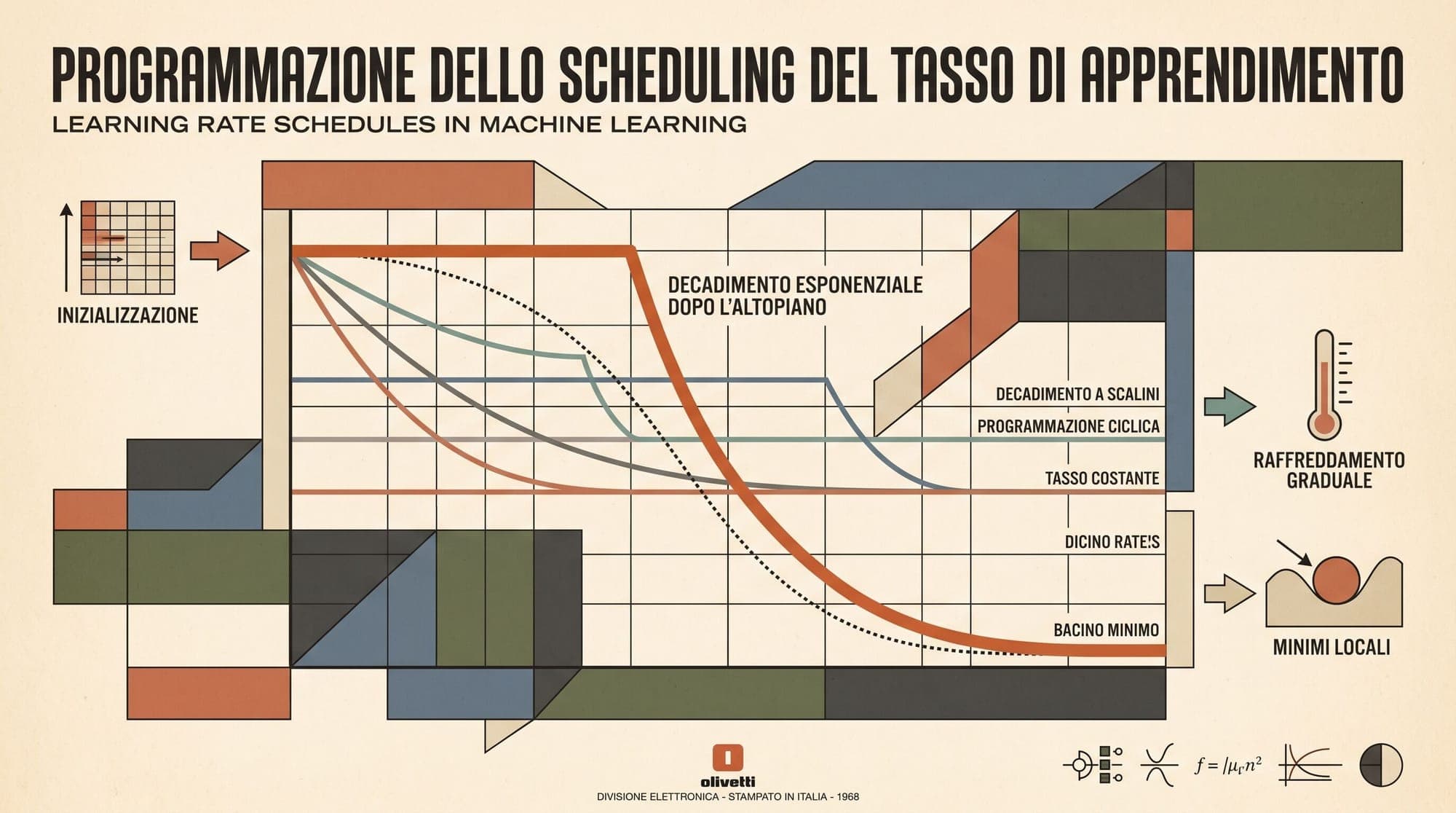
For years, foundation model pre-training adhered to a standard optimization convention: linear learning rate warmup followed by a full-horizon cosine decay. Adopted across GPT-3, PaLM, Chinchilla, and LLaMA, cosine annealing provided stable convergence across diverse parameter scales. However, it introduced a severe structural limitation: the learning rate schedule is rigidly tied to a fixed, upfront token budget. If a team decides to extend pre-training mid-run, branch into domain-specific variants, or test intermediate capabilities, cosine decay forces difficult trade-offs between optimization instability and wasted compute.

The Warmup-Stable-Decay (WSD) learning rate schedule, introduced by Shengding Hu and researchers at Tsinghua University and ModelBest in the MiniCPM project, and subsequently analyzed in studies by Ibrahim et al., Hägele et al., and Gu et al., has established itself as the modern standard for large language model pre-training. By decoupling the exploration phase from the convergence phase, WSD enables open-ended continual pre-training, dynamic compute scaling, and high-impact data annealing.

The Rigidity Bottleneck of Cosine Annealing

In classical cosine annealing, the learning rate $\eta(t)$ at optimization step $t$ across a total predetermined budget $T$ is governed by:

$$\eta(t) = \eta_{min} + \frac{1}{2}(\eta_{max} - \eta_{min})\left(1 + \cos\left(\frac{t}{T}\pi\right)\right)$$

While smooth, this functional form imposes several operational constraints:

1. Fixed Token Commitment: The entire training budget $T$ must be committed before the first gradient step. If additional clean data or compute becomes available at step $T$, extending training requires either re-warming the learning rate (which introduces catastrophic gradient variance and performance spikes) or continuing at the minimum floor $\eta_{min}$, where parameter updates stall.
2. Intermediate Checkpoint Suboptimality: Checkpoints saved mid-run (e.g., at $0.5 \times T$) reflect an un-decayed learning rate state and perform poorly on downstream evaluations compared to a model natively trained for $0.5 \times T$ steps.
3. Inflexible Data Mixing: Because the learning rate is continually decreasing, high-quality data injected late in the schedule is processed with a tiny step size, limiting the network's ability to restructure its internal representations.

The Three Regimes of Warmup-Stable-Decay

WSD replaces the global curve with three explicitly separated training regimes:

$$\eta(t) = \begin{cases} \eta_{max} \cdot \frac{t}{W} & 0 \le t < W \\ \eta_{max} & W \le t < S \\ \eta_{min} + (\eta_{max} - \eta_{min}) \cdot f(t - S) & S \le t \le T \end{cases}$$

Here, $W$ denotes warmup steps, $S$ denotes the start of the decay phase, and $T$ is the final step.

1. Warmup Phase ($0 \le t < W$)

Occupying 1% to 2% of the initial training budget, the warmup phase ramps the learning rate linearly from 0 to $\eta_{max}$. This conditions the optimizer's second-moment accumulators in AdamW and guides weights away from chaotic initialization points without destabilizing layer activations.

2. Stable Phase ($W \le t < S$)

The stable phase accounts for the vast majority of training (typically 80% to 90% of total tokens). During this phase, $\eta(t)$ remains fixed at peak learning rate $\eta_{max}$. The model maintains maximum exploration velocity across the loss surface, accumulating general syntactic, semantic, and factual representations.

Because the learning rate is constant, the training run can continue indefinitely. A team can train for 1 trillion, 5 trillion, or 10 trillion tokens along a single persistent optimization trajectory without committing to an end date.

3. Decay Phase ($S \le t \le T$)

When the target token budget or data distribution target is reached, the decay phase reduces the learning rate over the final 10% to 15% of steps down to $\eta_{min}$ (often $0.1 \times \eta_{max}$ or 0).

Common decay functions $f(t - S)$ include:

• Linear Decay: $f(\Delta t) = 1 - \frac{\Delta t}{T - S}$
• Cosine Decay: $f(\Delta t) = \frac{1}{2}\left(1 + \cos\left(\frac{\Delta t}{T - S}\pi\right)\right)$
• Exponential / Inverse-Square Root: Rapidly reducing the learning rate by a factor of 10x to 100x within the first half of the decay window.

During this final decay window, validation loss drops rapidly, matching or outperforming an equivalent model trained from scratch with a global cosine schedule over the same total compute budget.

Loss Landscape Dynamics: The River Valley Perspective

The empirical puzzle of WSD is why maintaining a high learning rate across 90% of training does not harm final convergence. During the stable phase, validation loss appears to plateau early, yet triggering the decay phase immediately unlocks dramatic loss drops.

Theoretical work by Gu et al. models this behavior through the lens of a River Valley loss landscape. The high-dimensional optimization surface is decomposed into two dominant components:

1. Hill Directions (High Curvature): Steep, narrow canyon walls representing high-frequency parameter interactions.
2. River Directions (Low Curvature): A long, gently sloping valley floor representing the global progression toward optimal representations.

Under a high constant learning rate $\eta_{max}$, gradient noise causes the AdamW optimizer to oscillate violently between the canyon walls (the "hill" modes). This cross-sectional oscillation generates an elevated baseline loss, creating the illusion that the model has stopped learning.

However, the large step size simultaneously maximizes the model's velocity along the valley floor (the "river" modes). The network makes rapid, unhindered progress through the principal parameter space.

When the decay phase begins:

• The reduction in learning rate suppresses transverse gradient variance.
• The optimizer drops out of the canyon wall oscillations and settles into the lowest point of the valley floor.
• The "hill" component of the loss vanishes linearly with the decrease in learning rate, realizing the cumulative representation gains achieved during the stable phase.

Data Annealing and Checkpoint Branching

The operational power of WSD lies in data annealing and branching architectures.

High-Quality Data Annealing

In modern foundation model pipelines (such as LLaMA 3 and MiniCPM), pre-training data is stratified by quality:

• Stable Phase: Trained on massive, diverse, web-scale corpora (e.g., Common Crawl, filtered web documents) to build broad knowledge and linguistic fluency.
• Decay Phase: The data mix is abruptly shifted to high-value tokens, including curated synthetic reasoning dialogues, formal mathematics, verified code repositories, and high-density textbook data.

Because the learning rate drops precisely as this high-quality distribution is introduced, the model crystallizes its final parameters around high-reasoning features without catastrophic forgetting of the broad world knowledge acquired during the stable phase.

Zero-Waste Checkpoint Branching

Under cosine decay, evaluating whether a model benefits from specialized data requires launching an entire pre-training run from step 0.

Under WSD, a single foundation run serves as a persistent backbone. At any point (for instance, at 2T tokens or 5T tokens), engineers can branch off the stable checkpoint and run parallel decay experiments:

• Branch A: Decayed on coding and algorithmic problem sets for developer tools.
• Branch B: Decayed on multi-lingual and translation corpora.
• Branch C: Decayed on domain-specific biomedical or financial data.

Each branch requires only 10% to 15% of the total compute budget, turning foundation model exploration into a modular, multi-fork pipeline.

Implementation Guidelines

A standard PyTorch learning rate scheduler implementing WSD with configurable decay profiles can be structured as follows:

import math
from torch.optim.lr_scheduler import _LRScheduler

class WarmupStableDecayLR(_LRScheduler):
    """
    Warmup-Stable-Decay (WSD) Learning Rate Scheduler.
    
    Phases:
      1. Warmup: Linear increase from 0 to max_lr over warmup_steps.
      2. Stable: Constant max_lr from warmup_steps to decay_start_step.
      3. Decay: Cosine, linear, or 1-sqrt decay from decay_start_step to total_steps.
    """
    def __init__(
        self,
        optimizer,
        warmup_steps: int,
        decay_start_step: int,
        total_steps: int,
        min_lr_ratio: float = 0.0,
        decay_type: str = "cosine",
        last_epoch: int = -1
    ):
        self.warmup_steps = warmup_steps
        self.decay_start_step = decay_start_step
        self.total_steps = total_steps
        self.min_lr_ratio = min_lr_ratio
        self.decay_type = decay_type
        super().__init__(optimizer, last_epoch)

    def get_lr(self):
        step = self.last_epoch
        if step < self.warmup_steps:
            alpha = step / max(1, self.warmup_steps)
            return [base_lr * alpha for base_lr in self.base_lrs]
        elif step < self.decay_start_step:
            return [base_lr for base_lr in self.base_lrs]
        else:
            decay_steps = self.total_steps - self.decay_start_step
            progress = min(1.0, (step - self.decay_start_step) / max(1, decay_steps))
            
            if self.decay_type == "cosine":
                decay_factor = self.min_lr_ratio + 0.5 * (1.0 - self.min_lr_ratio) * (1.0 + math.cos(math.pi * progress))
            elif self.decay_type == "linear":
                decay_factor = self.min_lr_ratio + (1.0 - self.min_lr_ratio) * (1.0 - progress)
            elif self.decay_type == "sqrt":
                decay_factor = self.min_lr_ratio + (1.0 - self.min_lr_ratio) * (1.0 - math.sqrt(progress))
            else:
                raise ValueError(f"Unsupported decay type: {self.decay_type}")
                
            return [base_lr * decay_factor for base_lr in self.base_lrs]

Empirical Rules of Thumb

• Warmup Ratio: 1% to 2% of total planned steps is sufficient to prevent early training divergence in bfloat16 mixed-precision regimes.
• Decay Length: 10% to 15% of total steps balances computational cost with full convergence. Decaying over less than 5% can cause underfitting on the target data mix, while decaying over more than 20% sacrifices stable exploration time.
• Terminal Learning Rate: Decaying to zero ($\eta_{min} = 0$) or near-zero ($0.01 \times \eta_{max}$) yields the lowest final perplexity, while retaining a 10% floor ($0.1 \times \eta_{max}$) facilitates subsequent fine-tuning stages.

Sources

• MiniCPM: Unveiling the Potential of Small Language Models with Scalable Training Strategies - Hu et al., 2024 (arXiv:2404.06395)
• Understanding Warmup-Stable-Decay Learning Rates: A River Valley Loss Landscape Perspective - Gu et al., 2024 (arXiv:2410.05192)
• Simple and Scalable Strategies to Continually Pre-train Large Language Models - Ibrahim et al., 2024 (arXiv:2403.08763)
• Scaling Laws and Compute-Optimal Training via Constant Learning Rates - Hägele et al., 2024 (arXiv:2405.18392)
• SGDR: Stochastic Gradient Descent with Warm Restarts - Loshchilov & Hutter, 2016 (arXiv:1608.03983)