The Fisher Information Matrix and Natural Gradient Descent: How Information Geometry, Riemannian Manifolds, and Curvature Invariance Reshape Neural Optimization

Standard gradient descent operates under an implicit, often unexamined assumption: that parameter space is Euclidean. When an optimizer updates network weights via $\theta_{t+1} = \theta_t - \eta \nabla_\theta \mathcal{L}(\theta)$, it calculates the direction of steepest descent within an arbitrary coordinate system. If the network is reparameterized without changing its input-output mapping, the Euclidean gradient vector changes direction and magnitude, leading to different optimization trajectories and variable convergence rates.

Natural gradient descent, introduced to neural networks by Shun-ichi Amari (1998), resolves this parameterization dependence. By treating the neural network as a statistical model that defines a family of probability distributions, natural gradient optimization replaces the Euclidean metric with a Riemannian metric tensor derived from information geometry: the Fisher Information Matrix (FIM).

The Parameterization Problem in Euclidean Optimization

In standard first-order optimization, the update direction is defined by the steepest descent problem under an $L_2$ norm constraint on the parameter displacement vector $d\theta$:

$$\min_{d\theta} \mathcal{L}(\theta + d\theta) \quad \text{subject to} \quad \|d\theta\|_2^2 \le \epsilon^2$$

Using a first-order Taylor expansion $\mathcal{L}(\theta + d\theta) \approx \mathcal{L}(\theta) + \nabla_\theta \mathcal{L}(\theta)^T d\theta$, the solution yields $d\theta \propto -\nabla_\theta \mathcal{L}(\theta)$.

The fundamental limitation of this formulation is that the constraint $\|d\theta\|_2^2 = \sum_i (d\theta_i)^2 \le \epsilon^2$ measures distance purely in coordinate space. Consider an invertible, smooth parameter transformation $\phi = g(\theta)$. By the chain rule, the gradient in the new coordinate system is:

$$\nabla_\phi \mathcal{L} = J^T \nabla_\theta \mathcal{L}$$

where $J = \frac{\partial \theta}{\partial \phi}$ is the Jacobian matrix of the coordinate transformation. A standard gradient step in $\phi$-coordinates produces:

$$\phi_{t+1} = \phi_t - \eta \nabla_\phi \mathcal{L} = \phi_t - \eta J^T \nabla_\theta \mathcal{L}$$

Mapping this update back to the original $\theta$-coordinates via $\theta = g^{-1}(\phi)$ does not yield $\theta_t - \eta \nabla_\theta \mathcal{L}(\theta)$. The optimization path is coupled to the arbitrary choice of coordinates rather than the underlying predictive function.

Information Geometry and the Statistical Manifold

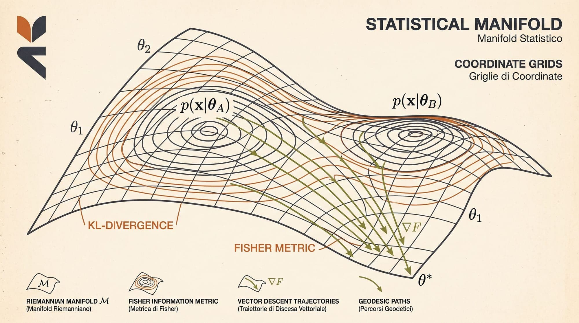
In deep learning, a parameterized model defines a conditional probability distribution $p_\theta(y|x)$ over target outputs $y$ given inputs $x$. The set of all such distributions forms a statistical manifold:

$$\mathcal{M} = \left\{ p_\theta(y|x) : \theta \in \Theta \subseteq \mathbb{R}^D \right\}$$

Points on this manifold are probability distributions, not parameter vectors. To measure the true distance between two nearby models parameterized by $\theta$ and $\theta + d\theta$, the natural metric is the Kullback-Leibler (KL) divergence averaged over the data distribution $p_{data}(x)$:

$$D_{KL}(p_\theta \parallel p_{\theta + d\theta}) = \mathbb{E}_{x \sim p_{data}(x)} \left[ \int p_\theta(y|x) \log \frac{p_\theta(y|x)}{p_{\theta + d\theta}(y|x)} \, dy \right]$$

The KL divergence is invariant to any invertible reparameterization of $\theta$ because the probability densities $p(y|x)$ remain unchanged.

Mathematical Derivation of the Fisher Information Matrix

To understand local distances on the manifold, consider the second-order Taylor expansion of $D_{KL}(p_\theta \parallel p_{\theta + d\theta})$ with respect to the parameter perturbation $d\theta$ around $d\theta = 0$.

Let $f(d\theta) = D_{KL}(p_\theta \parallel p_{\theta + d\theta})$. Evaluating the zeroth and first-order terms:

1. At $d\theta = 0$, $D_{KL}(p_\theta \parallel p_\theta) = 0$, so the zeroth-order term vanishes: $f(0) = 0$.
2. Because $D_{KL}(P \parallel Q) \ge 0$ with a global minimum at $P = Q$, the gradient with respect to $d\theta$ at $d\theta = 0$ is zero: $\nabla_{d\theta} f(0) = 0$.

The first non-vanishing term is the second-order Hessian matrix $\nabla_{d\theta}^2 f(0)$. Differentiating inside the expectation:

$$\nabla_{d\theta} \log p_{\theta + d\theta}(y|x) \Big|_{d\theta = 0} = \nabla_\theta \log p_\theta(y|x)$$

$$\nabla_{d\theta}^2 \log p_{\theta + d\theta}(y|x) \Big|_{d\theta = 0} = \nabla_\theta^2 \log p_\theta(y|x)$$

Expanding the log-ratio inside the divergence:

$$D_{KL}(p_\theta \parallel p_{\theta + d\theta}) = -\mathbb{E}_{x \sim p_{data}} \mathbb{E}_{y \sim p_\theta(\cdot|x)} \left[ \log p_{\theta + d\theta}(y|x) - \log p_\theta(y|x) \right]$$

Taking the second derivative with respect to $d\theta$:

$$\nabla_{d\theta}^2 D_{KL}(p_\theta \parallel p_{\theta + d\theta}) \Big|_{d\theta = 0} = -\mathbb{E}_{x \sim p_{data}} \mathbb{E}_{y \sim p_\theta(\cdot|x)} \left[ \nabla_\theta^2 \log p_\theta(y|x) \right]$$

Using the Bartlett identity, differentiating the normalization condition $\int p_\theta(y|x) dy = 1$ twice yields the equivalence between the negative expected Hessian of the log-likelihood and the outer product of score vectors:

$$\mathbb{E}_{y \sim p_\theta(\cdot|x)} \left[ -\nabla_\theta^2 \log p_\theta(y|x) \right] = \mathbb{E}_{y \sim p_\theta(\cdot|x)} \left[ \nabla_\theta \log p_\theta(y|x) \nabla_\theta \log p_\theta(y|x)^T \right]$$

This defines the Fisher Information Matrix $F(\theta) \in \mathbb{R}^{D \times D}$:

$$F(\theta) = \mathbb{E}_{x \sim p_{data}} \mathbb{E}_{y \sim p_\theta(\cdot|x)} \left[ \nabla_\theta \log p_\theta(y|x) \nabla_\theta \log p_\theta(y|x)^T \right]$$

The local KL divergence between two infinitesimally close models is therefore given by the quadratic form:

$$D_{KL}(p_\theta \parallel p_{\theta + d\theta}) = \frac{1}{2} d\theta^T F(\theta) d\theta + \mathcal{O}(\|d\theta\|^3)$$

Chentsov's Theorem (1982) established that the Fisher Information Matrix defines the unique Riemannian metric tensor (up to a scaling factor) on the statistical manifold that is invariant under sufficient statistics and Markov embeddings.

Natural Gradient Descent Formulation

With the Riemannian metric established, steepest descent on the statistical manifold is formulated by constraining the change in model distribution via KL divergence rather than Euclidean parameter distance:

$$\min_{d\theta} \mathcal{L}(\theta + d\theta) \quad \text{subject to} \quad D_{KL}(p_\theta \parallel p_{\theta + d\theta}) \le c$$

Substituting the first-order approximation for the loss and the quadratic approximation for the KL divergence:

$$\min_{d\theta} \left\{ \mathcal{L}(\theta) + \nabla_\theta \mathcal{L}(\theta)^T d\theta \right\} \quad \text{subject to} \quad \frac{1}{2} d\theta^T F(\theta) d\theta \le c$$

Formulating the Lagrangian with multiplier $\lambda > 0$:

$$\mathcal{L}_{Lagrange}(d\theta, \lambda) = \nabla_\theta \mathcal{L}(\theta)^T d\theta + \lambda \left( \frac{1}{2} d\theta^T F(\theta) d\theta - c \right)$$

Taking the derivative with respect to $d\theta$ and setting it to zero:

$$\nabla_\theta \mathcal{L}(\theta) + \lambda F(\theta) d\theta = 0 \implies d\theta = -\frac{1}{\lambda} F(\theta)^{-1} \nabla_\theta \mathcal{L}(\theta)$$

Setting the learning rate $\eta = \frac{1}{\lambda}$, the natural gradient update rule is:

$$\theta_{t+1} = \theta_t - \eta F(\theta_t)^{-1} \nabla_\theta \mathcal{L}(\theta_t)$$

The vector $\tilde{\nabla} \mathcal{L}(\theta) = F(\theta)^{-1} \nabla_\theta \mathcal{L}(\theta)$ is termed the natural gradient.

Proof of Reparameterization Invariance

To verify that natural gradient descent is invariant to coordinate transformations, let $\phi = g(\theta)$ with Jacobian $J = \frac{\partial \theta}{\partial \phi}$.

Transforming the score function:

$$\nabla_\phi \log p(y|x, \phi) = J^T \nabla_\theta \log p(y|x, \theta)$$

The Fisher Information Matrix in $\phi$-coordinates becomes:

$$F_\phi = \mathbb{E} \left[ \nabla_\phi \log p \nabla_\phi \log p^T \right] = J^T F_\theta J$$

The loss gradient transforms as $\nabla_\phi \mathcal{L} = J^T \nabla_\theta \mathcal{L}$. Computing the natural gradient in $\phi$-coordinates:

$$\tilde{\nabla}_\phi \mathcal{L} = F_\phi^{-1} \nabla_\phi \mathcal{L} = (J^T F_\theta J)^{-1} J^T \nabla_\theta \mathcal{L} = J^{-1} F_\theta^{-1} (J^T)^{-1} J^T \nabla_\theta \mathcal{L} = J^{-1} F_\theta^{-1} \nabla_\theta \mathcal{L} = J^{-1} \tilde{\nabla}_\theta \mathcal{L}$$

Multiplying both sides by $J$:

$$J \tilde{\nabla}_\phi \mathcal{L} = \tilde{\nabla}_\theta \mathcal{L}$$

By the chain rule, $d\theta = J d\phi$. The parameter updates describe the exact same displacement in the space of predictive distributions, guaranteeing invariance to any smooth, invertible coordinate transformation to first order.

Natural Gradient vs. Generalized Gauss-Newton vs. Hessian

Natural gradient descent is closely connected to classical second-order optimization, but exhibits distinct geometric and numerical properties analyzed by James Martens (2020).

Consider a network with output $f(x; \theta)$ trained under negative log-likelihood loss:

$$\mathcal{L}(\theta) = \mathbb{E}_{(x, y) \sim p_{data}} [-\log p(y | f(x; \theta))]$$

The true Hessian of this loss function with respect to parameters $\theta$ decomposes into two components via the chain rule:

$$\nabla_\theta^2 \mathcal{L}(\theta) = \mathbb{E}_{(x, y)} \left[ J_f^T \nabla_f^2 L(f, y) J_f \right] + \mathbb{E}_{(x, y)} \left[ \sum_{k} \frac{\partial L}{\partial f_k} \nabla_\theta^2 f_k(x; \theta) \right]$$

where $J_f = \frac{\partial f}{\partial \theta}$ is the Jacobian of network outputs with respect to parameters.

1. The Generalized Gauss-Newton (GGN) Matrix: The first term dropped the second-order network derivatives $\nabla_\theta^2 f_k$. When the loss function $L(f, y)$ corresponds to the negative log-likelihood of an exponential family distribution (such as softmax cross-entropy or mean squared error), the expectation of the GGN under the model's predictive distribution $y \sim p_\theta(y|x)$ exactly equals the Fisher Information Matrix:

$$F(\theta) = GGN(\theta) = \mathbb{E}_{x \sim p_{data}} \left[ J_f^T \nabla_f^2 L(f, y) J_f \right]$$

1. Curvature Stability: While the true Hessian $\nabla_\theta^2 \mathcal{L}(\theta)$ can have negative eigenvalues in non-convex regions (leading unconstrained Newton steps toward saddle points or local maxima), the Fisher Information Matrix is an expectation of outer products:

$$v^T F(\theta) v = \mathbb{E} \left[ (v^T \nabla_\theta \log p_\theta)^2 \right] \ge 0 \quad \forall v$$

The FIM is guaranteed to be positive semi-definite (PSD) everywhere on the parameter manifold. Natural gradient steps always move in a descent direction for the loss.

The Empirical Fisher vs. True Fisher Dilemma

In practical implementations, calculating the true Fisher Information Matrix requires computing expectations over model predictions:

$$F(\theta) = \mathbb{E}_{x \sim p_{data}} \left[ \sum_{y} p_\theta(y|x) \nabla_\theta \log p_\theta(y|x) \nabla_\theta \log p_\theta(y|x)^T \right]$$

Because sampling from $p_\theta(y|x)$ or summing over all output classes adds computational overhead, many empirical studies historically substituted the "Empirical Fisher" matrix $\bar{F}(\theta)$:

$$\bar{F}(\theta) = \frac{1}{N} \sum_{i=1}^N \nabla_\theta \log p_\theta(y_i|x_i) \nabla_\theta \log p_\theta(y_i|x_i)^T$$

where $y_i$ is the actual ground truth training label rather than a sample from $p_\theta(y|x_i)$.

In a critical analysis, Frederik Kunstner, Lukas Balles, and Philipp Hennig (2019) demonstrated that the Empirical Fisher is not a valid approximation of either the Fisher Information Matrix or the Hessian:

• Lack of Second-Order Information: The Empirical Fisher coincides with the true Fisher if and only if the model's predictive distribution perfectly matches the data distribution ($p_\theta(y|x) = p_{data}(y|x)$), which occurs only at zero training error.
• Pathological Scaling: Away from the optimum, the Empirical Fisher is simply the sample covariance of the gradients around zero. In directions where gradients are large, $\bar{F}$ scales quadratically with gradient magnitude, causing the update step $\bar{F}^{-1} \nabla \mathcal{L}$ to damp updates precisely where strong progress is required.
• Adaptive Optimizers (Adam) Are Not Natural Gradient: Popular diagonal adaptive optimizers like Adam scale updates by $\sqrt{v_t}$, where $v_t$ is an exponential moving average of squared empirical gradients $\nabla \mathcal{L}_i^2$. Because they utilize empirical data labels rather than model expectation sampling, they do not perform natural gradient descent or true metric-tensor Riemannian optimization.

Scalable Approximations in Modern Deep Learning

For large language models with billions of parameters ($D \ge 10^9$), storing the full $D \times D$ Fisher matrix requires petabytes of memory, and inverting it via $\mathcal{O}(D^3)$ matrix inversion is computationally intractable.

To make natural gradient practical, structural approximations partition and factorize the curvature:

1. Block-Diagonal Approximations

Treating parameters across different layers as mutually independent replaces the full FIM with a block-diagonal matrix, where each block corresponds to a single layer's weight matrix $W_l \in \mathbb{R}^{d_{out} \times d_{in}}$.

2. Kronecker-Factored Approximate Curvature (K-FAC)

Introduced by James Martens and Roger Grosse (2015), K-FAC approximates each layer's Fisher block $F_l$ as the Kronecker product ($\otimes$) of two smaller matrices:

$$F_l \approx A_{l-1} \otimes S_l$$

where:

• $A_{l-1} = \mathbb{E}[a_{l-1} a_{l-1}^T]$ is the covariance of input activations to layer $l$.
• $S_l = \mathbb{E}[s_l s_l^T]$ is the covariance of pre-activation loss derivatives for layer $l$.

Using the Kronecker inversion identity $(A \otimes B)^{-1} = A^{-1} \otimes B^{-1}$, inverting an otherwise intractable $(d_{in} d_{out}) \times (d_{in} d_{out})$ matrix reduces to inverting two small matrices of size $d_{in} \times d_{in}$ and $d_{out} \times d_{out}$:

$$(A_{l-1} \otimes S_l)^{-1} \text{vec}(\nabla_{W_l} \mathcal{L}) = \text{vec}\left( S_l^{-1} \nabla_{W_l} \mathcal{L} A_{l-1}^{-1} \right)$$

This formulation scales natural gradient preconditioning to deep neural networks with minimal computational overhead per training step.

3. Beyond K-FAC: Shampoo and Matrix Orthogonalization

Recent post-Adam optimization methods extend these geometric insights. Shampoo (Gupta et al., 2018) and Distributed Shampoo (Anil et al., 2020) compute roots of layer-wise activation and gradient covariance matrices to construct block-wise preconditioned tensor updates. Modern matrix optimizers like Muon (Bernstein et al., 2025) employ Newton-Schulz iterations to directly orthogonalize parameter updates, enforcing spectral bounds on updates across weight matrices.

Summary

Natural gradient descent re-anchors optimization from coordinate-space mechanics to the intrinsic geometry of probability distributions. By preconditioning parameter updates with the inverse Fisher Information Matrix:

1. Parameter updates become invariant to arbitrary reparameterizations and scale shifts.
2. The optimizer measures trajectory step lengths in Kullback-Leibler divergence on the statistical manifold rather than Euclidean distance.
3. The Fisher Information Matrix serves as a guaranteed positive semi-definite surrogate for the Hessian, matching the Generalized Gauss-Newton matrix under log-likelihood objectives.
4. Structured factorizations like K-FAC, Shampoo, and spectral preconditioning bridge information-theoretic natural gradients with the extreme scale requirements of modern foundation model pre-training.

Sources

• Amari, S. (1998). Natural gradient works efficiently in learning. Neural Computation, 10(2), 251-276. https://doi.org/10.1162/089976698300017746
• Martens, J. (2020). New insights and perspectives on the natural gradient method. Journal of Machine Learning Research, 21(146), 1-76. https://jmlr.org/papers/v21/17-678.html / https://arxiv.org/abs/1412.1193
• Kunstner, F., Balles, L., & Hennig, P. (2019). Limitations of the empirical Fisher approximation for natural gradient descent. Advances in Neural Information Processing Systems (NeurIPS 2019). https://arxiv.org/abs/1905.12558
• Pascanu, R., & Bengio, Y. (2014). Revisiting Natural Gradient for Deep Networks. International Conference on Learning Representations (ICLR 2014). https://arxiv.org/abs/1301.3583
• Martens, J., & Grosse, R. (2015). Optimizing Neural Networks with Kronecker-factored Approximate Curvature. International Conference on Machine Learning (ICML 2015). https://arxiv.org/abs/1503.05671
• Chentsov, N. N. (1982). Statistical Decision Rules and Optimal Inference. Translations of Mathematical Monographs, American Mathematical Society. https://doi.org/10.1007/978-94-009-6987-2