RWKV Architecture: How Receptance Weighted Key Value Decay Combines RNN Efficiency with Transformer Parallelizability

The dominant paradigm in natural language processing relies on the Transformer architecture, which calculates scaled dot-product self-attention across all token pairs in a sequence. While self-attention provides strong in-context retrieval and representation capacity, it imposes quadratic computational and memory complexity, scaling as O(N^2) with sequence length N during training and generating a continuously expanding Key-Value (KV) cache during autoregressive inference.

Traditional Recurrent Neural Networks (RNNs), such as Long Short-Term Memory (LSTM) networks and Gated Recurrent Units (GRUs), maintain constant O(1) memory complexity per generation step by compressing history into a fixed-size hidden state. However, classic RNNs suffer from sequential training bottlenecks: the hidden state at step t depends non-linearly on the hidden state at step t-1, preventing parallel computation across sequence positions during backpropagation.

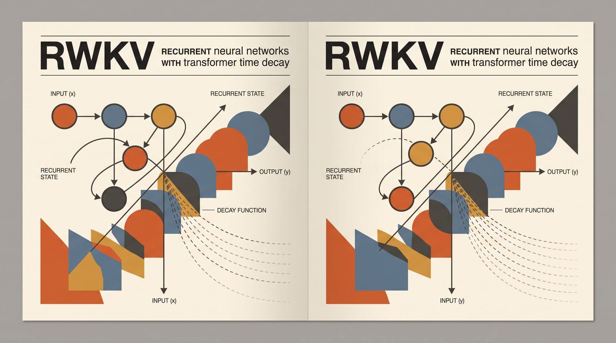
The Receptance Weighted Key Value (RWKV) architecture, introduced by Bo Peng and the open-source RWKV community in arXiv:2305.13048, bridges this divide. By formulating attention as a linear recurrence with channel-wise exponential time decay, RWKV achieves the dual properties of Transformer-style parallelized training and RNN-style constant-memory inference.

The Four Core Primitives

RWKV replaces standard multi-head self-attention with a linear formulation governed by four vector representations:

Receptance (R): Computed as $r_t = \sigma(W_r x'_t)$ , where $\sigma$ denotes the sigmoid function and $x'_t$ is a time-shifted token representation. Receptance acts as a dynamic acceptance gate, determining the degree to which past accumulated context is factored into the current output.
Weight / Time Decay (W): A learnable, channel-wise negative decay vector $w \in \mathbb{R}^d$ . The term $e^{-w}$ determines the continuous exponential rate at which historical tokens fade from memory per feature dimension.
Key (K): Computed as $k_t = W_k x'_t$ , projecting the input into a key vector analogous to the Keys in Transformer attention.
Value (V): Computed as $v_t = W_v x'_t$ , projecting the input into the candidate feature representation.

Before linear projections are calculated, RWKV applies a causal 1D temporal mixing operation termed Token-Shift (or Time-Shift). For any input vector sequence $x_t$ , the shifted representation $x'_t$ is a channel-wise linear interpolation between the current token and the preceding token:

$x'_t = x_t \odot \mu + x_{t-1} \odot (1 - \mu)$

where $\mu \in \mathbb{R}^d$ is a learnable interpolation vector per projection branch ( $R, K, V$ ). Token-shift provides each layer with immediate local context from the previous time step without introducing full recurrent matrix multiplication.

The Mathematical Equivalence of Parallel and Recurrent Modes

The foundation of RWKV is the Weighted Key-Value (WKV) operator. In self-attention, the attention matrix requires computing $\text{softmax}(Q K^T / \sqrt{d}) V$ . RWKV replaces the pairwise dot-product query-key matching with an element-wise decaying sum inspired by the Attention Free Transformer (arXiv:2105.14103).

RWKV Time-Mixing and Recurrence Schematic

Time-Parallel Mode (Training)

During training, all tokens $t \in [1, T]$ are known simultaneously. The WKV output vector at sequence position $t$ , denoted as $\text{wkv}_t$ , is calculated across all preceding positions $i < t$ :

$\text{wkv}_t = \frac{\sum_{i=1}^{t-1} \exp(-(t - 1 - i)w + k_i) \odot v_i + \exp(u + k_t) \odot v_t}{\sum_{i=1}^{t-1} \exp(-(t - 1 - i)w + k_i) + \exp(u + k_t)}$

Here, $w \in \mathbb{R}_{\ge 0}^d$ is the learnable channel-wise decay vector, and $u \in \mathbb{R}^d$ is a learnable bonus vector assigned specifically to the current token $t$ to allow the model to attend strongly to the present input without distorting the historical decay curve.

Because the historical terms decay purely as a function of relative distance $(t - 1 - i)w$ , the numerator and denominator sums can be executed in parallel across the sequence using custom CUDA associative scan kernels or 1D depthwise causal convolutions, achieving $O(T)$ computational complexity over sequence length $T$ .

Time-Sequential Mode (Inference)

During autoregressive generation, computing the full summation across all past tokens would reintroduce linear time growth per generated token. Because the decay operator is linear and exponential, the summation decomposes cleanly into two running state vectors: a numerator accumulator $a_t \in \mathbb{R}^d$ and a denominator accumulator $b_t \in \mathbb{R}^d$ .

At generation step $t$ , given the input $x_t$ and the previous state $(a_{t-1}, b_{t-1})$ :

Calculate current projections:

$x'_t = x_t \odot \mu_x + x_{t-1} \odot (1 - \mu_x)$ $r_t = \sigma(W_r x'_t), \quad k_t = W_k x'_t, \quad v_t = W_v x'_t$

Compute WKV output for step $t$ :

$\text{wkv}_t = \frac{a_{t-1} + \exp(u + k_t) \odot v_t}{b_{t-1} + \exp(u + k_t)}$

Update recurrent state for step $t+1$ :

$a_t = \exp(-w) \odot a_{t-1} + \exp(k_t) \odot v_t$ $b_t = \exp(-w) \odot b_{t-1} + \exp(k_t)$

Compute layer output:

$o_t = W_o (r_t \odot \text{wkv}_t)$

In this recurrent form, step $t$ requires only $O(1)$ arithmetic operations and exactly $2d$ floating-point values for state retention. The model does not retain past activations, eliminating KV cache memory expansion regardless of context length.

Block Architecture: Time-Mixing and Channel-Mixing

Each RWKV layer consists of two sub-blocks: a Time-Mixing block (replacing self-attention) and a Channel-Mixing block (replacing the feedforward network). Both blocks utilize pre-layer normalization and residual connections.

[Input Tensor x_t]
       |
       +------------------------------------+
       |                                    |
   LayerNorm                            Residual
       |                                    |
  Time-Mixing Block                         |
  (Token-Shift -> R, K, V -> WKV -> R*WKV)  |
       |                                    |
       +-----------------(+) <--------------+
       |
       +------------------------------------+
       |                                    |
   LayerNorm                            Residual
       |                                    |
 Channel-Mixing Block                       |
 (Token-Shift -> R, K -> GeLU/ReLU^2 -> R*K)|
       |                                    |
       +-----------------(+) <--------------+
       |
[Output Tensor x_{t+1}]

Channel-Mixing Block Mechanics

The Channel-Mixing block handles cross-channel feature transformations through a gated non-linear activation:

Token Shift: $x'_{cm, t} = x_t \odot \mu_{cm} + x_{t-1} \odot (1 - \mu_{cm})$
Receptance & Key Projections:

$r_t = \sigma(W_{r, cm} x'_{cm, t})$ $k_t = \max(W_{k, cm} x'_{cm, t}, 0)^2 \quad \text{(Squared ReLU / GeLU)}$

Value Projection & Gated Modulation:

$o_{cm, t} = r_t \odot (W_{v, cm} k_t)$

The gating mechanism in both blocks allows RWKV to dynamically suppress or amplify representations channel-by-channel, preventing gradient explosion and maintaining stability during deep network training.

Evolution Across Architecture Generations

The RWKV architecture has evolved through several iterations to increase expressive power while maintaining strict linear inference:

RWKV-4: The Vector-State Baseline

Described in arXiv:2305.13048, RWKV-4 utilizes scalar decay per channel and vector-valued hidden states ( $a_t, b_t \in \mathbb{R}^d$ ). While computationally lightweight, storing information in independent scalar channels limits the model's ability to maintain complex inter-channel associations across long sequences.

RWKV-5 (Eagle): Matrix-Valued Multi-Head States

Introduced in arXiv:2404.05892, Eagle expands the recurrent state from 1D vectors to multi-headed 2D matrix states:

$S_{h, t} = \exp(-w_h) \odot S_{h, t-1} + k_{h, t}^T v_{h, t}$

where $S_{h, t} \in \mathbb{R}^{d_k \times d_v}$ represents the hidden state matrix for head $h$ . This modification transforms RWKV from a channel-wise weighted average into a generalized linear attention mechanism closely related to Gated Linear Attention (arXiv:2312.06635) and State Space Duality (arXiv:2405.21060), vastly improving multi-token associative recall.

RWKV-6 (Finch): Dynamic Recurrence and Context-Aware Token-Shift

Finch (arXiv:2404.05892) replaces static learned parameters with data-dependent dynamic mechanisms:

Dynamic Token-Shift: The interpolation parameter $\mu$ becomes a function of the current input vector via a low-rank projection: $\mu(x_t) = \text{sigmoid}(W_a \tanh(W_b x_t))$ .
Dynamic Time Decay: The decay rate $w$ is generated dynamically per token, allowing the model to selectively retain or erase past state based on content: $w_t = \text{softplus}(W_{w} \tanh(W_{a} x_t))$ .

Architectural and Serving Trade-Offs

When comparing RWKV against standard Transformer and State Space Model (SSM) deployments, several operational trade-offs emerge:

Memory Footprint and KV Cache Elimination

In standard Transformer serving (e.g., Llama or Mistral), KV cache VRAM consumption scales linearly with sequence length, batch size, and layer count:

$\text{VRAM}_{\text{KV}} = 2 \times L \times H_{kv} \times d_{head} \times B \times N \times \text{bytes\_per\_element}$

For an 8B Transformer handling a batch of 32 requests at 32k context in FP16, the KV cache alone consumes over 64 GB of GPU memory. In contrast, RWKV requires a constant memory buffer per sequence:

$\text{VRAM}_{\text{RWKV}} = L \times H \times d_k \times d_v \times B \times \text{bytes\_per\_element}$

This memory footprint remains identical whether generating token 10 or token 100,000, enabling large-batch inference and on-device deployment without VRAM exhaustion.

Prefill and Decoding Latency Profiles

Decoding (Generation): RWKV processes each generated token in constant $O(1)$ time, maintaining uniform step latency regardless of how long the conversation has progressed. Standard Transformers experience increasing per-token decoding latency as self-attention attends over an expanding KV cache.
Prefill (Prompt Processing): During prefill, standard Transformers execute highly optimized FlashAttention-3 kernels on GPUs. RWKV executes parallel associative scans (Chunk-WKV kernels), matching Transformer prefill throughput while avoiding memory allocation for KV caches.

The Information-Theoretic Bottleneck

The primary limitation of linear recurrent architectures, including RWKV and Mamba, lies in the information capacity of the fixed-size hidden state. Because the recurrent state must compress an arbitrary sequence length into a constant-dimensional tensor, linear models face fundamental capacity limits on tasks requiring exact multi-hop associative recall across long distances (Multi-Query Associative Recall, arXiv:2312.04927).

While full quadratic attention can retrieve any arbitrary token pair through uncompressed dot products, RWKV relies on its continuous decay and dynamic state update to approximate relevant context. For structured reasoning, general conversational generation, and streaming data processing, RWKV achieves accuracy competitive with equivalently sized Transformers while delivering substantial efficiency gains during deployment.