RWKV Architecture: How Receptance Weighted Key Value Combines RNN Linear Inference with Transformer Parallel Training

Transformer architectures dominate modern large language model design, yet standard multi-head self-attention exhibits an inherent operational bottleneck: sequence processing complexity scales quadratically ( $O(N^2)$ ) with context length during training, while autoregressive generation requires maintaining an expanding key-value (KV) cache that consumes $O(N)$ memory per request. Conversely, traditional recurrent neural networks (RNNs) such as LSTMs and GRUs evaluate sequences in constant $O(1)$ time and memory per step during inference, but suffer from strict sequential dependencies during backpropagation that prevent efficient parallel training on modern accelerator hardware.

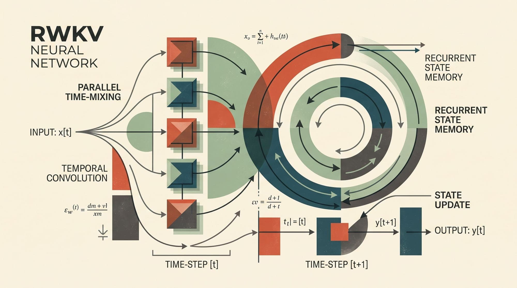
The Receptance Weighted Key Value (RWKV) architecture reconciles these competing paradigms. By reformulating attention as a linear recurrent state update governed by exponential time decay, RWKV achieves parallelized, GPU-efficient $O(N)$ training while operating as a constant-memory $O(1)$ RNN during sequential generation.

RWKV Linear Attention and Recurrence Architecture

The Fundamental Mathematical Duality: Parallel and Recurrent Modes

At the core of RWKV is the mathematical equivalence between linear attention with causal exponential decay and linear recurrent state space transitions.

In standard softmax self-attention, the output vector for token $t$ is computed across all previous tokens $i \le t$ as:

$\text{Attn}(Q, K, V)_t = \sum_{i=1}^{t} \frac{\exp(q_t^\top k_i)}{\sum_{j=1}^{t} \exp(q_t^\top k_j)} v_i$

The non-linear softmax normalizer couples every query token to every key token independently, necessitating the materialization of an $N \times N$ attention matrix or retaining every historical key and value tensor in memory.

RWKV replaces the pairwise dot-product query-key score $\exp(q_t^\top k_i)$ with an additive decay kernel and a gating mechanism termed Receptance ( $R$ ). In the baseline RWKV-4 formulation, the weighted key-value operator ( $WKV$ ) for token $t$ computes:

$WKV_t = \frac{\sum_{i=1}^{t-1} \exp(-(t-1-i)w + k_i) \odot v_i + \exp(u + k_t) \odot v_t}{\sum_{i=1}^{t-1} \exp(-(t-1-i)w + k_i) + \exp(u + k_t)}$

where:

$w \in \mathbb{R}^d$ is a learnable, non-negative channel-wise time-decay vector.
$u \in \mathbb{R}^d$ is a bonus weight vector applied exclusively to the current token $t$ to preserve immediate token attention without artificial decay.
$k_i$ and $v_i$ represent linear projections of the input sequence.

The Parallel Training Formulation

During training, when the full sequence of length $N$ is available simultaneously, the denominator and numerator of $WKV$ represent causal 1D convolutions with an exponential decay filter $\exp(-w \cdot \Delta t)$ . This operation can be computed across the sequence via parallel associative prefix scans (cumulative sums in log-space) or custom GPU CUDA kernels, achieving $O(N)$ computational complexity per sequence without ever allocating an $N \times N$ attention grid.

The Recurrent Inference Formulation

During sequential autoregressive generation, RWKV unrolls directly into a pure linear recurrent state machine. By factoring the exponential decay recursively, the cumulative numerator state $a_t \in \mathbb{R}^d$ and denominator normalizer state $b_t \in \mathbb{R}^d$ update step-by-step in $O(1)$ time and memory:

$\begin{aligned} WKV_t &= \frac{a_{t-1} + \exp(u + k_t) \odot v_t}{b_{t-1} + \exp(u + k_t)} \\ a_t &= \exp(-w) \odot a_{t-1} + \exp(k_t) \odot v_t \\ b_t &= \exp(-w) \odot b_{t-1} + \exp(k_t) \end{aligned}$

At inference time, the model maintains only the hidden vectors $a_t$ and $b_t$ . The physical KV cache is eliminated entirely: inference memory consumption and generation latency remain strictly constant whether generating token 10 or token 100,000.

Core Building Blocks: Time-Mixing and Channel-Mixing

An RWKV layer consists of two sequential sub-blocks analogous to the attention and feed-forward network (FFN) blocks of a Transformer: Time-Mixing and Channel-Mixing.

1. Token-Shifting (Time-Shift Operator)

Both blocks apply a parameter-free temporal interpolation mechanism called Token-Shifting. Before computing linear projections, the input vector $x_t$ at step $t$ is linearly blended with the input vector from the previous step $x_{t-1}$ :

$\begin{aligned} r_t &= W_r \cdot \left(\mu_r \odot x_t + (1 - \mu_r) \odot x_{t-1}\right) \\ k_t &= W_k \cdot \left(\mu_k \odot x_t + (1 - \mu_k) \odot x_{t-1}\right) \\ v_t &= W_v \cdot \left(\mu_v \odot x_t + (1 - \mu_v) \odot x_{t-1}\right) \end{aligned}$

where $\mu_r, \mu_k, \mu_v \in [0, 1]^d$ are learnable interpolation vectors. Token-shifting provides local n-gram context mixing directly at the input stage of each layer, allowing subsequent operations to capture local feature dependencies with minimal computational overhead.

2. Time-Mixing Block

The Time-Mixing block produces the layer's temporal communication. After evaluating $WKV_t$ , the output is modulated by the Receptance vector $r_t$ passed through a sigmoid activation:

$\text{Output}_{\text{time}} = W_o \cdot \left(\sigma(r_t) \odot WKV_t\right)$

The Receptance vector acts as an acceptance gate: $\sigma(r_t) \approx 0$ suppresses historical accumulation, whereas $\sigma(r_t) \approx 1$ allows the decayed key-value history to pass to subsequent layers.

3. Channel-Mixing Block

The Channel-Mixing block handles cross-channel feature transformations, replacing the conventional Transformer MLP:

$\begin{aligned} r_t' &= W_{r'} \cdot \left(\mu_{r'} \odot x_t + (1 - \mu_{r'}) \odot x_{t-1}\right) \\ k_t' &= W_{k'} \cdot \left(\mu_{k'} \odot x_t + (1 - \mu_{k'}) \odot x_{t-1}\right) \\ \text{Output}_{\text{channel}} &= \sigma(r_t') \odot \left(W_{v'} \cdot \text{ReLU}(k_t')^2\right) \end{aligned}$

Here, squared ReLU activations ( $\text{ReLU}(x)^2$ ) introduce non-linear expressivity, while the gated receptance $\sigma(r_t')$ controls information flow through the feed-forward projection.

Architectural Evolution: RWKV-4 to Eagle and Finch

The RWKV architecture has undergone substantial iterative improvements to address expressivity bottlenecks in early linear recurrent designs.

RWKV-4 (Baseline Formulation)

State Representation: Vector-valued state ( $a_t, b_t \in \mathbb{R}^d$ ).
Decay Schedule: Static, channel-wise learnable parameter vector $w$ .
Receptance Activation: Sigmoid gating $\sigma(r_t)$ .
Limitation: Vector states restricted the total information capacity that could be stored across long sequences, leading to degraded performance on multi-hop associative retrieval tasks.

RWKV-5 "Eagle" (Matrix-Valued Multi-Head States)

Introduced in the Eagle and Finch paper, RWKV-5 restructured the internal recurrent state from 1D vectors into multi-headed 2D matrix states:

Matrix State Formulation: For $H$ heads each of dimension $d_h = d / H$ , the recurrent state becomes a matrix $S_t^{(h)} \in \mathbb{R}^{d_h \times d_h}$ , updated via outer product accumulation:

$S_t^{(h)} = \exp(-w^{(h)}) \odot S_{t-1}^{(h)} + k_t^{(h)\top} v_t^{(h)}$

Multi-Head Normalization: Group normalization is applied across individual heads before output projection.
Attention Gating: Replaces standard sigmoid gating with SiLU-based output modulation and removes the denominator normalizer to stabilize multi-head updates.

RWKV-6 "Finch" (Data-Dependent Dynamic Recurrence)

RWKV-6 introduced data-dependent dynamic mechanisms that allow the model to vary its decay rates and token mixing dynamically based on current context:

Dynamic Time Decay ( $w_t$ ): The decay rate is no longer a static parameter. Instead, $w_t$ is computed dynamically per token via low-rank adapter projections (LoRA):

$w_t = w_{\text{base}} + \tanh\left(x_t W_{w1}\right) W_{w2}$ This allows the network to selectively flush its memory state when encountering topic transitions or retain specific tokens across arbitrary context spans.

Dynamic Token-Shift (ddlerp): Interpolation weights $\mu(x_t)$ are computed dynamically from input features, enabling context-sensitive local mixing.

Complexity and Operational Scaling

A comparative analysis of computational complexity and memory footprint across modern architectures reveals the structural differences between attention and recurrence:

Standard Softmax Attention (Transformer): Training compute scales as $O(N^2)$ with $O(N^2)$ activation memory. Autoregressive inference requires $O(N)$ compute per step and an $O(N)$ expanding KV cache. Training is fully parallelizable.
FlashAttention-2: Training compute scales as $O(N^2)$ with $O(N)$ memory through tiling. Inference remains $O(N)$ compute per step and requires an $O(N)$ expanding KV cache. Training is fully parallelizable.
State Space Models (Mamba / S4): Training compute scales linearly as $O(N)$ with $O(N)$ memory. Inference runs in constant $O(1)$ compute per step with a constant $O(1)$ state representation. Training is fully parallelizable.
RWKV-4: Training compute scales linearly as $O(N)$ with $O(N)$ memory. Inference runs in constant $O(1)$ compute per step with a $2d$ vector state. Training is fully parallelizable via WKV prefix scans.
RWKV-5 / RWKV-6: Training compute scales linearly as $O(N)$ with $O(N)$ memory. Inference runs in constant $O(1)$ compute per step with an $H \cdot d_h^2$ matrix state. Training is fully parallelizable.

Engineering Strengths and Trade-Offs

1. Zero KV Cache Growth on Edge Devices

Because RWKV maintains a fixed-size internal state matrix regardless of sequence depth, memory consumption remains deterministic. A 7B parameter RWKV-6 model requires approximately 14 GB of VRAM in FP16 for the model weights, plus a negligible ~10-20 MB recurrent state buffer, whether processing prompt token 1 or token 500,000. This eliminates the out-of-memory (OOM) failures common to long-context Transformer deployments on consumer hardware.

2. Continuous Real-Time Streaming and Low TTFT

In continuous streaming applications (such as speech processing, robotics control, or unbounded event log monitoring), RWKV processes input tokens incrementally without recalculating historical attention matrices or reloading multi-gigabyte KV caches.

3. Trade-Off: Associative Recall vs. Fixed Memory Capacity

By compressing infinite historical context into a finite matrix state $S_t \in \mathbb{R}^{d_h \times d_h}$ , linear recurrent models inherently trade lossless token retrieval for memory efficiency. While Transformers can directly access historical tokens via pairwise softmax dot products, RWKV must encode patterns into recurrent state transitions. Although RWKV-6 data-dependent decay mitigates this gap on standard synthetic benchmarks (such as Needle-In-A-Haystack up to 128k tokens), dense multi-variable lookups across vast contexts remain an area of ongoing architectural optimization.