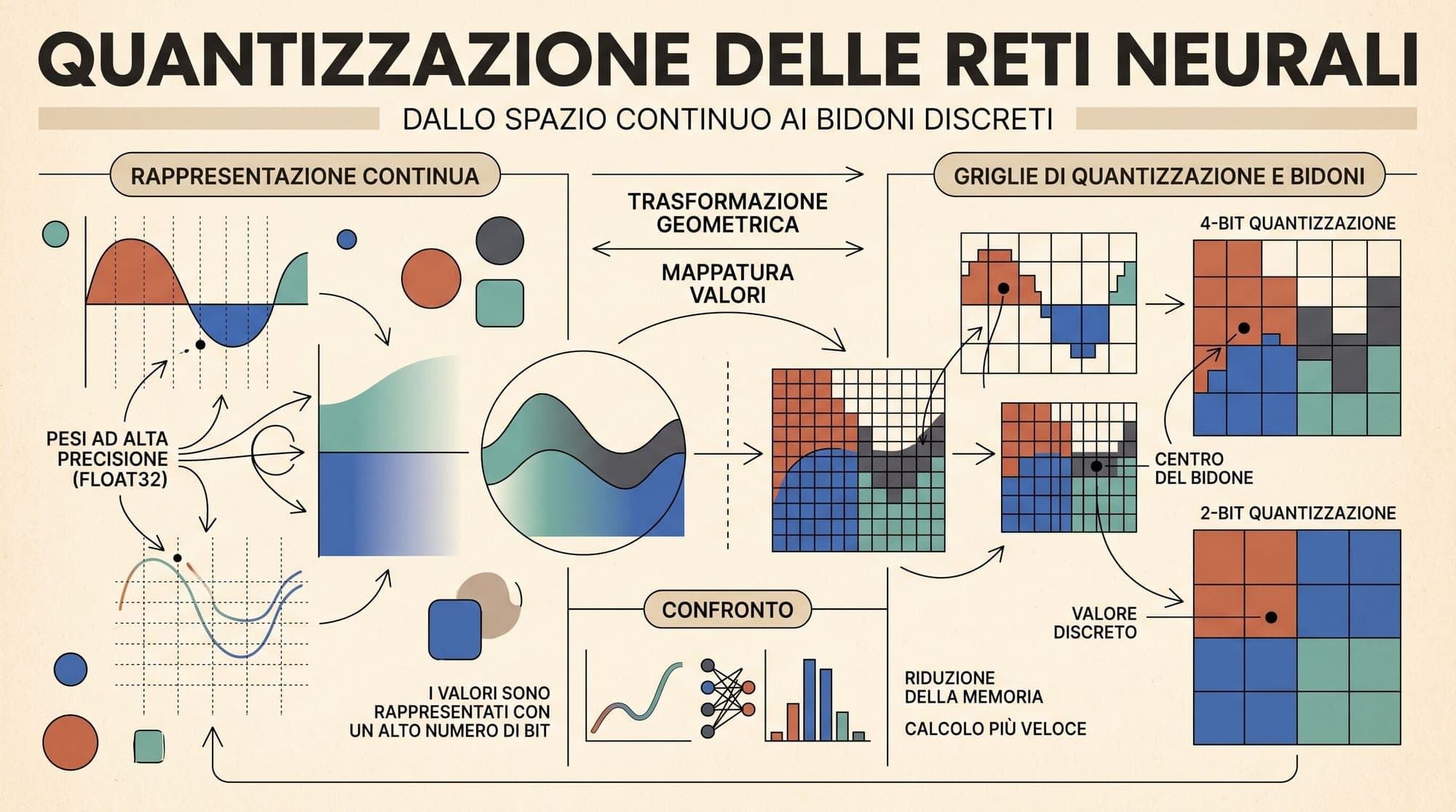
Quantization-Aware Training in Large Language Models: How Fake Quantization, STE, and Learned Step Sizes Preserve Low-Bit Accuracy

Quantization-Aware Training (QAT) is a model compression paradigm that integrates precision loss directly into the training or fine-tuning graph. While Post-Training Quantization (PTQ) calibrates fixed floating-point weights without updating underlying network parameters, QAT simulates the numerical discretization of weights, activations, and key-value (KV) caches during both forward and backward passes. This closed-loop optimization forces neural network weights to co-adapt to discrete integer lattices, preventing the catastrophic perplexity degradation that typically occurs when compressing large language models (LLMs) down to 4-bit, 3-bit, or 2-bit representations.

Understanding QAT requires analyzing the mathematical mechanics of uniform quantization, the non-differentiable nature of rounding operators, surrogate gradient estimators, learnable grid scaling, and modern data-efficient distillation frameworks tailored for multi-billion parameter architectures.

The PTQ Accuracy Cliff and Activation Outliers

Post-Training Quantization techniques such as GPTQ and AWQ minimize layer-wise output reconstruction error using second-order Taylor expansions or activation-aware salience weighting. In 8-bit weight-only or 4-bit weight-only regimes, PTQ preserves near-lossless perplexity across standard language benchmarks.

However, PTQ encounters fundamental limitations when two conditions arise:

Low-Bit Weight Regimes (≤3 bits): The distance between available quantization grid points grows exponentially as bit-width drops. Second-order error compensations can no longer resolve the accumulated rounding residuals across deep transformer stacks.
Joint Weight-Activation Quantization (W8A8, W4A4): As shown by Dettmers et al. (2022), transformer hidden states develop high-magnitude outlier channels in specific feature dimensions once model parameter scale exceeds 6.7 billion parameters. These activation outliers exhibit dynamic ranges up to 100 times larger than normal tokens. Quantizing activations to uniform low-bit integers using static PTQ scales truncates normal tokens or squashes all non-outlier features into identical integer bins.

QAT resolves these bottlenecks by maintaining continuous parameter trajectories that migrate across quantization boundaries during training, discovering weight configurations that remain resilient to quantized activation tensors.

The Mathematics of Uniform Quantization

Uniform affine quantization maps a continuous floating-point tensor $x \in \mathbb{R}$ to a discrete $b$ -bit integer grid $[q_{\min}, q_{\max}]$ . For unsigned representations, $q_{\min} = 0$ and $q_{\max} = 2^b - 1$ ; for signed two's complement representations, $q_{\min} = -2^{b-1}$ and $q_{\max} = 2^{b-1} - 1$ .

The mapping from real values $x$ to quantized integers $q$ is governed by two parameters: a positive real-valued scale factor $S$ and an integer zero-point $Z$ :

$q = \text{clamp}\left(\left\lfloor \frac{x}{S} \right\rceil + Z, \, q_{\min}, \, q_{\max}\right)$

where $\lfloor \cdot \rceil$ denotes the round-to-nearest-integer operator, and the clamp function is defined as:

$\text{clamp}(v, a, b) = \min(\max(v, a), b)$

The dequantization operator reconstructs an approximate real value $\hat{x} \approx x$ :

$\hat{x} = S \cdot (q - Z)$

In symmetric quantization, the zero-point $Z$ is fixed to zero ( $Z = 0$ ), mapping the symmetric real range $[-\alpha, \alpha]$ directly across the signed integer bounds:

$S = \frac{\alpha}{2^{b-1} - 1}, \quad \hat{x} = S \cdot \text{clamp}\left(\left\lfloor \frac{x}{S} \right\rceil, -2^{b-1}, 2^{b-1}-1\right)$

Straight-Through Estimator and Fake Quantization Workflow

Fake Quantization and the Non-Differentiability Bottleneck

Executing actual integer arithmetic during model training is computationally impractical: backpropagation requires continuous floating-point gradients to perform parameter updates via optimizers like AdamW. Furthermore, the derivative of the rounding function $\lfloor u \rceil$ is zero everywhere except at half-integers, where it is completely undefined:

$\frac{d \lfloor u \rceil}{d u} = 0 \quad (\forall u \notin \mathbb{Z} + 0.5)$

If standard automatic differentiation were applied directly to quantized weights, the gradient of the loss $\mathcal{L}$ with respect to the continuous weight $w$ would evaluate to zero:

$\frac{\partial \mathcal{L}}{\partial w} = \frac{\partial \mathcal{L}}{\partial \hat{w}} \cdot \frac{\partial \hat{w}}{\partial w} = \frac{\partial \mathcal{L}}{\partial \hat{w}} \cdot 0 = 0$

To bypass this vanishing gradient barrier, Jacob et al. (2018) established the concept of fake quantization (also known as simulated quantization). Under fake quantization:

Continuous "shadow weights" $w$ are stored and updated in high precision (FP32 or BF16).
In the forward pass, a fake-quantization operator $Q_{\text{fake}}(w)$ clamps and rounds the weight into the discrete grid, but immediately scales it back into floating-point representation $\hat{w}$ .
Matrix multiplications are computed using these discretized values $\hat{w}$ .
In the backward pass, a surrogate gradient replaces the ill-defined derivative of the rounding operator.

The Straight-Through Estimator (STE)

The foundational surrogate gradient for discrete neural operations is the Straight-Through Estimator (STE), first introduced by Hinton (2012) and formalized by Bengio et al. (2013).

The STE models the non-differentiable rounding operator as an identity mapping during the backward pass while retaining the clipping boundary indicator:

$\frac{\partial \hat{w}}{\partial w} \approx \begin{cases} 1 & \text{if } \alpha \le w \le \beta \\ 0 & \text{otherwise} \end{cases}$

Under this approximation, the gradient flows directly from the output tensor back to the continuous shadow weights:

$\frac{\partial \mathcal{L}}{\partial w} = \frac{\partial \mathcal{L}}{\partial \hat{w}} \cdot \mathbb{I}(\alpha \le w \le \beta)$

Where $\mathbb{I}(\cdot)$ is the indicator function. The shadow weights absorb tiny fractional updates across training steps. When accumulated gradient steps push a shadow weight past a rounding threshold $(k + 0.5)S$ , its discretized value $\hat{w}$ jumps to the next grid point in subsequent forward passes.

Learned Step Size Quantization (LSQ)

Early QAT systems treated the clipping bounds $[\alpha, \beta]$ and step size $S$ as static hyper-parameters computed from tensor min/max statistics or exponential moving averages. However, static boundaries create an unresolvable trade-off: wide boundaries reduce clipping distortion at the expense of coarse rounding bins, while narrow boundaries preserve fine resolution at the expense of severe truncation.

Esser et al. (2020) solved this problem with Learned Step Size Quantization (LSQ). LSQ reparameterizes the quantization scale factor $S$ as an explicit continuous parameter that is jointly optimized alongside network weights via backpropagation.

Let normalized weight $v = \frac{w}{S}$ . The symmetric quantized representation is:

$\bar{v} = \text{clamp}\left(\left\lfloor v \right\rceil, -Q_N, Q_P\right)$

$\hat{w} = \bar{v} \cdot S$

Applying the chain rule to the step size $S$ yields an analytical gradient:

$\frac{\partial \hat{w}}{\partial S} = \begin{cases} -\frac{w}{S} + \left\lfloor \frac{w}{S} \right\rceil & \text{if } -Q_N < \frac{w}{S} < Q_P \\ -Q_N & \text{if } \frac{w}{S} \le -Q_N \\ Q_P & \text{if } \frac{w}{S} \ge Q_P \end{cases}$

This gradient provides continuous feedback to the step size:

If weights within the grid suffer from rounding errors, the residual $-\frac{w}{S} + \lfloor \frac{w}{S} \rceil$ nudges $S$ to minimize discretization noise.
If significant weight mass falls outside the grid, the saturated terms $(-Q_N, Q_P)$ push $S$ to expand, enlarging the dynamic range to prevent clipping saturation.

Overcoming LLM Scale: Data-Free and Distillation QAT

Applying naive QAT to foundation language models presents two severe operational challenges:

Compute Overhead: Re-training a 70B parameter model across hundreds of billions of tokens with fake quantization requires massive GPU cluster allocations.
Dataset Accessibility and Drift: Proprietary pre-training mixtures are rarely available to downstream deployment engineers, and fine-tuning on narrow open corpora can trigger catastrophic forgetting.

To eliminate these barriers, researchers developed data-free and distillation-guided QAT frameworks:

LLM-QAT (Data-Free Knowledge Distillation)

Liu et al. (2023) proposed LLM-QAT, which removes dependency on external training corpora by utilizing the original unquantized model as both a synthetic data generator and a teacher network.

+-------------------------------------------------------------+
|               Unquantized Teacher Model                     |
|           (Generates Synthetic Text Prompts)                |
+-------------------------------------------------------------+
                               |
               Token Sequence Context (x_1...x_t)
                               |
            +------------------+------------------+
            |                                     |
            v                                     v
+-----------------------+             +-----------------------+
| Unquantized Teacher   |             | Fake-Quantized Student|
| FP16 Forward Pass     |             | (Weights, Act, KV)    |
+-----------------------+             +-----------------------+
            |                                     |
    Logits P(y|x)                         Logits Q(y|x)
            |                                     |
            +------------------+------------------+
                               |
                               v
                     KL Divergence Loss:
               L_KD = D_KL( P(y|x) || Q(y|x) )
                               |
                               v
            STE + LSQ Backpropagation on Student

Synthetic Data Generation: The frozen full-precision teacher model generates diverse token sequences using open-ended sampling.
Multi-Component Discretization: The student model inserts fake quantizers across three distinct targets: linear projection weights, intermediate activation tensors, and attention key-value (KV) cache buffers.
Cross-Entropy Distillation: The student optimizes the Kullback-Leibler (KL) divergence between teacher and student logit distributions:

$\mathcal{L}_{\text{KD}} = \sum_{t=1}^T D_{\text{KL}}\left(P_{\text{teacher}}(\cdot \mid x_{<t}) \,\|\, P_{\text{student}}(\cdot \mid x_{<t})\right)$

Because the student mimics the teacher's exact output distribution on model-generated data, the model retains general reasoning capabilities without human-labeled datasets.

Efficient Parameter-Efficient QAT (OmniQuant and LR-QAT)

To reduce memory consumption during QAT, frameworks such as OmniQuant (Shao et al., 2023) and Low-Rank QAT freeze original model weights and optimize only equivalent mathematical transformations:

Learnable Equivalent Scaling (LES): Learns channel-wise scaling factors that migrate outlier dynamic range from activations into weight matrices prior to quantization.
Learnable Weight Clipping (LWC): Optimizes layer-wise clipping thresholds using mini-batch calibration datasets.

Activation Smoothing and KV Cache Quantization

While weight tensors have stationary distributions, activation tensors vary dynamically across different input sequences. Standard QAT architectures implement two complementary techniques to stabilize activation quantization:

Channel-Wise Smoothing Transformations

Drawing from SmoothQuant (Xiao et al., 2023), models apply a mathematically equivalent diagonal scaling matrix $s \in \mathbb{R}^d$ across linear layers before applying fake quantization:

$Y = (X \cdot \text{diag}(s)^{-1}) \cdot (\text{diag}(s) \cdot W) = \hat{X} \cdot \hat{W}$

The per-channel scaling factor balances dynamic ranges:

$s_j = \frac{\max(|X_j|)^\alpha}{\max(|W_j|)^{1-\alpha}}$

where $\alpha \in [0, 1]$ controls the proportion of quantization difficulty migrated from activations to weights. During QAT, $s_j$ can be initialized via activation profiling and fine-tuned alongside LSQ scale factors.

Quantized Key-Value Caching

In multi-turn generation and long-context inference, the KV cache dominates GPU High Bandwidth Memory (HBM). QAT applies fake quantization to key and value projections prior to storage in cache buffers:

$K_{\text{quant}} = Q_{\text{fake}}(X \cdot W_K), \quad V_{\text{quant}} = Q_{\text{fake}}(X \cdot W_V)$

Training the attention heads with quantized KV tensors forces the query projection $W_Q$ and attention softmax layers to become robust to the minor angular deviations introduced by low-precision key vectors.

Transitioning from Fake Quantization to Integer Kernels

Fake quantization operates entirely within floating-point emulators during training. Once training loss converges, the artifact is exported to target hardware runtimes through a four-stage compilation process:

Parameter Freezing: Shadow weights $w$ are rounded to their final integer states $q_w = \text{clamp}(\lfloor w/S_w \rceil, q_{\min}, q_{\max})$ , and scale factors $S_w, S_x$ are frozen into constant buffers.
Graph Rewriting: Fake quantization nodes are removed from the computational graph.
Integer Packing: For sub-8-bit formats (such as INT4 or INT2), consecutive integer indices are packed into contiguous bytes (e.g. two 4-bit values per uint8 byte).
Kernel Binding: Standard FP32 GEMM operations are replaced with hardware-accelerated integer matrix multiplication instructions:

NVIDIA Tensor Cores: mma.sync.aligned.m16n8k32.row.col (INT4/INT8 arithmetic).
ARM NEON / Apple Silicon: SDOT and UDOT dot-product instructions.
Inference Runtimes: Integration into vLLM, TensorRT-LLM, or Marlin execution backends.

Training Phase (Simulated Quantization):
[Continuous Shadow Weights w] 
         |
         v
[Fake Quant Operator: Q_fake(w) = S * round(w/S)] -> [FP16 Matrix Mul] -> [Loss & STE Gradients]
                                                                                |
                                                                                v
                                                             [AdamW Updates continuous w and S]

Export & Deployment Phase (Physical Quantization):
[Frozen w, S] -> [Round & Cast to INT4/INT8] -> [Packed Weight Buffer] -> [Hardware Integer Tensor Cores]

Comparative Evaluation: PTQ vs. QAT

Optimization Target: PTQ minimizes local layer-wise or block-wise reconstruction error, whereas QAT optimizes global task loss and end-to-end token cross-entropy.
Gradient Flow: PTQ operates without backpropagation, while QAT utilizes full-model surrogate gradient propagation via the Straight-Through Estimator.
Scale Optimization: PTQ relies on heuristic grid search or MSE clipping, whereas QAT optimizes step sizes dynamically via Learned Step Size Quantization (LSQ).
Compute and Data Requirements: PTQ executes in minutes on a single GPU with small calibration batches (128 to 512 samples). QAT requires moderate training budgets (GPU hours to days) using synthetic distillation or curated corpora.
Low-Bit Recovery: PTQ exhibits severe perplexity spikes below 4-bit representation. QAT maintains functional reasoning and benchmark accuracy down to 3-bit and 2-bit weight regimes.
Activation Outlier Handling: PTQ requires mixed-precision execution channels or dynamic per-token clipping. QAT natively reshapes weight manifolds to tolerate compressed activation representations.

Summary

Quantization-Aware Training bridges the gap between theoretical compression limits and operational deployment efficiency. By combining simulated discrete forward passes with the Straight-Through Estimator and Learned Step Sizes, QAT enables continuous optimizers to navigate discontinuous loss surfaces. Modern distillation architectures like LLM-QAT and low-rank parameter-efficient fine-tuning make QAT applicable to frontier language models without requiring access to original pre-training corpora or prohibitive supercomputing budgets.