Proximal Policy Optimization (PPO) in LLM Post-Training: Mathematical Foundations of Clipped Surrogate Objectives, Generalized Advantage Estimation, Value Network Architectures, and Adaptive KL Penalties

Reinforcement Learning from Human Feedback (RLHF) established modern alignment for instruction-following foundation models. While pre-training optimizes autoregressive language models to minimize next-token prediction loss over massive text corpora, standard cross-entropy loss cannot directly optimize for open-ended attributes such as helpfulness, harmlessness, mathematical correctness, or human preference.

To bridge this gap, modern post-training pipelines formalize sequence generation as a Markov Decision Process (MDP) and apply policy gradient reinforcement learning algorithms. Among these, Proximal Policy Optimization (PPO), originally introduced by Schulman et al. (2017) and adapted to foundation models by Stiennon et al. (2020) and Ouyang et al. (2022), serves as the foundational actor-critic alignment algorithm.

Understanding PPO requires examining its mathematical formulation: the four-model distributed infrastructure, per-token Kullback-Leibler (KL) reward shaping, Generalized Advantage Estimation (GAE), the clipped surrogate objective, and its computational trade-offs against newer reference-free or critic-free alternatives.

1. The MDP Formulation of Autoregressive Language Generation

In the RLHF setting, autoregressive text generation is framed as an episodic Markov Decision Process denoted by the tuple $(\mathcal{S}, \mathcal{A}, \mathcal{P}, \mathcal{R}, \gamma)$:

• State Space ($\mathcal{S}$): The state $s_t \in \mathcal{S}$ at step $t$ corresponds to the concatenation of the input prompt $x = (x_1, \dots, x_M)$ and all previously generated response tokens $y_{<t} = (y_1, \dots, y_{t-1})$. Thus, $s_t = (x, y_{<t})$.
• Action Space ($\mathcal{A}$): The action $a_t \in \mathcal{A}$ is the selection of the next token $y_t$ from the vocabulary $\mathcal{V}$, where $|\mathcal{V}|$ typically ranges between $32,000$ and $128,000$.
• Transition Dynamics ($\mathcal{P}$): State transitions are deterministic string concatenations: $s_{t+1} = (s_t, y_t) = (x, y_1, \dots, y_t)$. The episode terminates when the policy generates a special end-of-sequence token $\langle\text{EOS}\rangle$ or reaches a maximum length limit $T$.
• Policy ($\pi_\theta$): The parameterized language model defines a stochastic policy $\pi_\theta(a_t | s_t) = P(y_t | x, y_{<t})$.
• Discount Factor ($\gamma$): In language generation tasks, the standard discount factor is set to $\gamma = 1.0$, treating all generated tokens within the finite horizon $T$ with equal long-term weighting.

2. The Four-Model Distributed Architecture

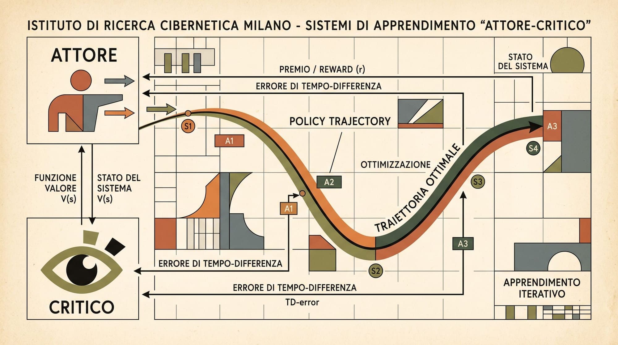
Standard PPO-based RLHF orchestrates four distinct language model instances during training:

                  +-----------------------------------+
                  |        Input Prompt (x)           |
                  +-----------------+-----------------+
                                    |
            +-----------------------+-----------------------+
            |                                               |
            v                                               v
  +-------------------+                           +-------------------+
  |   Active Policy   |                           |  Reference Model  |
  |   (Actor)         |                           |  (Frozen SFT)     |
  |   \pi_\theta(y|x) |                           |  \pi_{ref}(y|x)   |
  +---------+---------+                           +---------+---------+
            |                                               |
            | Generated Sequence y                          | Reference Logits
            | & Policy Logits                               |
            v                                               v
  +-------------------------------------------------------------------+
  |                    Per-Token KL Divergence Penalty                |
  |           r_{KL}(t) = -\beta * log(\pi_\theta / \pi_{ref})        |
  +---------------------------------+---------------------------------+
                                    |
            +-----------------------+-----------------------+
            |                                               |
            v                                               v
  +-------------------+                           +-------------------+
  |   Reward Model    |                           |   Critic Model    |
  |   (Frozen RM)     |                           |   (Value Function)|
  |   r_\psi(x, y)    |                           |   V_\phi(s_t)     |
  +---------+---------+                           +---------+---------+
            |                                               |
            +-----------------------+-----------------------+
                                    |
                                    v
                     +-----------------------------+
                     | Generalized Advantage       |
                     | Estimation (GAE)            |
                     | \hat{A}_t^{GAE(\gamma,\lambda)} |
                     +--------------+--------------+
                                    |
                                    v
                     +-----------------------------+
                     | PPO Clipped Optimization    |
                     | L^{CLIP}(\theta) + L^{VF}   |
                     +-----------------------------+

1. Active Policy / Actor ($\pi_\theta$): The primary model being trained. It generates the trajectory tokens $y_{1:T}$ and is updated using the clipped policy gradient objective. It is initialized from the Supervised Fine-Tuned (SFT) model.
2. Reference Model ($\pi_{\text{ref}}$): A static, frozen copy of the SFT checkpoint. It provides baseline token probabilities used to penalize the active policy when it deviates too far from the original distribution.
3. Reward Model ($R_\psi$): A frozen model trained on paired human or AI preference data $(x, y_w, y_l)$ under the Bradley-Terry preference model, defined by Bradley and Terry (1952) and Christiano et al. (2017):

$$P(y_w \succ y_l | x) = \sigma(R_\psi(x, y_w) - R_\psi(x, y_l)) = \frac{1}{1 + e^{-(R_\psi(x, y_w) - R_\psi(x, y_l))}}$$ The scalar reward $r_\psi(x, y) \in \mathbb{R}$ evaluates the full response.

1. Value Network / Critic ($V_\phi$): A parameterized model that maps intermediate states $s_t$ to expected cumulative future rewards $V_\phi(s_t) \in \mathbb{R}$. It is typically initialized from the reward model architecture with a modified scalar head and updated via mean squared error against empirical return targets.

3. Reward Augmentation and Per-Token KL Regularization

A foundational challenge in reinforcement learning for language models is "reward hacking" or policy collapse: without regularization, an unconstrained policy $\pi_\theta$ exploits quirks and misspecifications in the reward model $R_\psi$, generating nonsensical, repetitive, or adversarial strings that achieve high reward scores but lose linguistic coherence.

To prevent distribution shift away from the natural language manifold, PPO incorporates a Kullback-Leibler (KL) divergence penalty into the objective function:

$$\max_\theta \mathbb{E}_{x \sim \mathcal{D}, y \sim \pi_\theta(\cdot | x)} \left[ R_\psi(x, y) - \beta \, \mathbb{D}_{\text{KL}}\left(\pi_\theta(\cdot | x) \,\|\, \pi_{\text{ref}}(\cdot | x)\right) \right]$$

Because language generation occurs sequentially token by token, the full trajectory KL divergence can be decomposed into exact per-token penalties. The augmented token-level reward $R_t$ at step $t$ is formulated as:

$$R_t = \begin{cases} -\beta \left( \log \pi_\theta(y_t | x, y_{<t}) - \log \pi_{\text{ref}}(y_t | x, y_{<t}) \right) & \text{if } t < T \\ R_\psi(x, y) - \beta \left( \log \pi_\theta(y_T | x, y_{<T}) - \log \pi_{\text{ref}}(y_T | x, y_{<T}) \right) & \text{if } t = T \end{cases}$$

Here, $\beta > 0$ is the KL penalty coefficient.

Dynamic Adaptive KL Controller

While $\beta$ can remain constant, Ziegler et al. (2019) and Ouyang et al. (2022) introduced an adaptive proportional controller that dynamically adjusts $\beta$ after each training iteration to track a target KL divergence $d_{\text{targ}}$:

$$d_t = \mathbb{D}_{\text{KL}}\left(\pi_\theta(\cdot | x) \,\|\, \pi_{\text{ref}}(\cdot | x)\right)$$

$$\beta_{k+1} = \begin{cases} \beta_k \left(1 + K_{\beta}\right) & \text{if } d_t > 1.5 \, d_{\text{targ}} \\ \beta_k \left(1 - K_{\beta}\right) & \text{if } d_t < \frac{d_{\text{targ}}}{1.5} \\ \beta_k & \text{otherwise} \end{cases}$$

where $K_{\beta}$ is a proportional scaling factor (typically $0.1$). This adaptive rule ensures that if the policy begins exploiting the reward model, $\beta$ automatically increases to pull the policy back toward $\pi_{\text{ref}}$.

4. Generalized Advantage Estimation (GAE) in Language Horizons

To compute policy gradient updates, the actor requires an estimate of the advantage function $A(s_t, a_t) = Q(s_t, a_t) - V(s_t)$, which quantifies how much better taking action $a_t$ is compared to the average action at state $s_t$.

In language generation, directly using Monte Carlo returns yields high variance, while one-step Temporal Difference (TD) updates introduce high bias due to inaccuracies in the learned value network $V_\phi$. Generalized Advantage Estimation (GAE), developed by Schulman et al. (2015), balances this trade-off using an exponentially decaying sum of temporal difference residuals.

Temporal Difference Residual

The 1-step TD residual $\delta_t^V$ at token step $t$ is defined as:

$$\delta_t^V = R_t + \gamma V_\phi(s_{t+1}) - V_\phi(s_t)$$

where $V_\phi(s_{T+1}) \equiv 0$ at the terminal boundary. With discount factor $\gamma = 1.0$:

$$\delta_t^V = R_t + V_\phi(s_{t+1}) - V_\phi(s_t)$$

GAE Advantage Computation

The Generalized Advantage Estimator $\hat{A}_t^{\text{GAE}(\gamma, \lambda)}$ is defined as the exponentially weighted average of $k$-step advantage estimators:

$$\hat{A}_t^{\text{GAE}(\gamma, \lambda)} = \sum_{l=0}^{T-t-1} (\gamma \lambda)^l \delta_{t+l}^V = \sum_{l=0}^{T-t-1} \lambda^l \delta_{t+l}^V \quad (\text{for } \gamma = 1.0)$$

This formulation yields a clean backward recurrence relation:

$$\hat{A}_t^{\text{GAE}} = \delta_t^V + (\gamma \lambda) \hat{A}_{t+1}^{\text{GAE}}$$

The hyperparameter $\lambda \in [0, 1]$ controls the variance-bias continuum:

• $\lambda = 0$: $\hat{A}_t = \delta_t^V = R_t + \gamma V_\phi(s_{t+1}) - V_\phi(s_t)$ (lowest variance, highest bias from value function error).
• $\lambda = 1$: $\hat{A}_t = \sum_{l=0}^{T-t-1} R_{t+l} - V_\phi(s_t)$ (empirical Monte Carlo return minus baseline, zero bias, highest variance).

In modern LLM post-training systems (such as DeepSpeed-Chat, TRL, and Ray/vLLM RL pipelines), standard parameter choices are $\gamma = 1.0$ and $\lambda = 0.95$.

Advantage Normalization

To stabilize optimization across mini-batches of varying response lengths and prompt difficulties, advantages are standardized across the mini-batch:

$$\hat{A}_t \leftarrow \frac{\hat{A}_t - \mu(\hat{A})}{\sigma(\hat{A}) + \epsilon_{\text{norm}}}$$

where $\mu(\hat{A})$ and $\sigma(\hat{A})$ are the empirical mean and standard deviation computed across all valid token positions in the rollout batch, and $\epsilon_{\text{norm}} = 10^{-8}$.

5. The Clipped Surrogate Objective

Standard policy gradient methods compute gradients proportional to $\nabla_\theta \log \pi_\theta(a_t | s_t) \hat{A}_t$. Performing multiple epochs of stochastic gradient descent on the same rollout data under this standard objective leads to destructive, unconstrained parameter updates because the data distribution shifts away from the policy that collected the rollouts.

PPO resolves this by introducing the probability ratio:

$$r_t(\theta) = \frac{\pi_\theta(y_t | x, y_{<t})}{\pi_{\theta_{\text{old}}}(y_t | x, y_{<t})} = \exp\left( \log \pi_\theta(y_t | x, y_{<t}) - \log \pi_{\theta_{\text{old}}}(y_t | x, y_{<t}) \right)$$

where $\pi_{\theta_{\text{old}}}$ denotes the parameter state prior to the current multi-epoch update phase. At the start of rollout collection, $r_t(\theta) = 1.0$.

The Clipped Objective Formulation

The PPO clipped surrogate policy loss $L^{\text{CLIP}}(\theta)$ is defined as:

$$L^{\text{CLIP}}(\theta) = \hat{\mathbb{E}}_t \left[ \min\left( r_t(\theta) \hat{A}_t, \, \text{clip}(r_t(\theta), 1 - \epsilon, 1 + \epsilon) \hat{A}_t \right) \right]$$

where $\epsilon$ is a clipping threshold (typically $\epsilon \in [0.1, 0.2]$).

Mechanics of the Min Operator

The interaction between the probability ratio $r_t(\theta)$, advantage $\hat{A}_t$, and clipping operator handles positive and negative advantages symmetrically:

1. Positive Advantage ($\hat{A}_t > 0$): The token action performed better than average. The gradient pushes $r_t(\theta)$ higher to increase the probability of generating this token. However, once $r_t(\theta) > 1 + \epsilon$, the clipped term $\text{clip}(r_t(\theta), 1-\epsilon, 1+\epsilon)\hat{A}_t = (1+\epsilon)\hat{A}_t$ becomes active. The $\min$ operator takes this constant ceiling, dropping the gradient to zero and preventing excessive updates.
2. Negative Advantage ($\hat{A}_t < 0$): The token action performed worse than average. The gradient pushes $r_t(\theta)$ lower to decrease token probability. When $r_t(\theta) < 1 - \epsilon$, the clipped term $(1-\epsilon)\hat{A}_t$ is larger (less negative) than $r_t(\theta)\hat{A}_t$. The $\min$ operator selects the lower bound, flattening the gradient and preventing catastrophic probability collapses.

6. Value Function Optimization and Joint Objective

Simultaneously with actor optimization, the value network $V_\phi$ must be trained to predict the discounted return targets $V_t^{\text{targ}} = \hat{A}_t^{\text{GAE}} + V_{\phi_{\text{old}}}(s_t)$.

Value Loss with Clipping

To prevent large updates to the critic network from destabilizing policy evaluation, the value loss $L^{\text{VF}}(\phi)$ incorporates symmetric clipping:

$$V_\phi^{\text{clip}}(s_t) = V_{\phi_{\text{old}}}(s_t) + \text{clip}\left( V_\phi(s_t) - V_{\phi_{\text{old}}}(s_t), -\epsilon_v, \epsilon_v \right)$$

$$L^{\text{VF}}(\phi) = \frac{1}{2} \hat{\mathbb{E}}_t \left[ \max\left( \left( V_\phi(s_t) - V_t^{\text{targ}} \right)^2, \, \left( V_\phi^{\text{clip}}(s_t) - V_t^{\text{targ}} \right)^2 \right) \right]$$

Pre-Training Gradient Mixing (PTX Loss)

In Ouyang et al. (2022), the authors observed that optimizing solely on RLHF preference rewards caused degradation in standard academic benchmarks (the "alignment tax"). To mitigate this capability degradation, InstructGPT introduced an auxiliary supervised pre-training loss ($L^{\text{PTX}}$) directly into the policy gradient:

$$L^{\text{PTX}}(\theta) = \mathbb{E}_{x_{\text{pretrain}} \sim \mathcal{D}_{\text{pretrain}}} \left[ \log \pi_\theta(x_{\text{pretrain}}) \right]$$

The Complete Optimization Objective

Combining all components yields the full multi-task objective for the actor and critic:

$$\max_\theta \min_\phi \mathbb{E} \left<a href="s_t"> L^{\text{CLIP}}(\theta) - c_1 L^{\text{VF}}(\phi) + c_2 S[\pi_\theta</a> + \gamma_{\text{PTX}} L^{\text{PTX}}(\theta) \right]$$

where:

• $S\pi_\theta = -\sum_{a} \pi_\theta(a|s_t) \log \pi_\theta(a|s_t)$ is the entropy bonus to encourage exploration (often set to $0$ for large models).
• $c_1$ is the value loss coefficient (typically $0.5$ to $1.0$).
• $\gamma_{\text{PTX}}$ is the pre-training mixing coefficient (set between $0$ and $27.0$ in InstructGPT).

7. Systems Constraints, GPU Memory Budgets, and the Post-PPO Landscape

Deploying PPO in production requires substantial infrastructure. A single training worker must hold four full models in memory or stream them efficiently across high-bandwidth interconnects:

| Model Component | Parameter State | Optimizer State (AdamW) | Gradient Buffers | Activation Memory | | :--- | :--- | :--- | :--- | :--- | | Actor ($\pi_\theta$) | FP16/BF16 ($2 \times N$) | FP32 ($12 \times N$) | FP16/BF16 ($2 \times N$) | Dynamic (Sequence Length $\times$ Batch) | | Critic ($V_\phi$) | FP16/BF16 ($2 \times N$) | FP32 ($12 \times N$) | FP16/BF16 ($2 \times N$) | Dynamic | | Reference ($\pi_{\text{ref}}$) | FP16/BF16 ($2 \times N$) | None ($0$) | None ($0$) | Minimal (Forward Only) | | Reward ($R_\psi$) | FP16/BF16 ($2 \times N$) | None ($0$) | None ($0$) | Minimal (Forward Only) |

For a 70-billion parameter model, holding all four models requires over $800\text{ GB}$ of GPU VRAM before accounting for activation caching and KV caches during the rollout generation phase.

Comparison: PPO vs Modern Post-Training Paradigms

Due to the memory overhead and hyperparameter sensitivity of PPO, alternative post-training algorithms have emerged:

| Characteristic | Proximal Policy Optimization (PPO) | Direct Preference Optimization (DPO) | Group Relative Policy Optimization (GRPO) | Simple Preference Optimization (SimPO) | | :--- | :--- | :--- | :--- | :--- | | Core Architecture | 4 Models (Actor, Critic, Ref, Reward) | 2 Models (Actor, Ref) | 2 Models (Actor, Ref) + Rule Verifier | 1 Model (Actor Only) | | Explicit Critic Network | Yes ($V_\phi$ required) | No (Implicit reward derivation) | No (Group-normalized baseline) | No (Reference-free implicit reward) | | Optimization Type | Online on-policy RL | Offline pairwise preference | Online group-sampled on-policy RL | Offline length-normalized preference | | Primary Use Case | Multi-step reasoning with learned reward models | General conversational alignment and style | Mathematical and reasoning tasks with verifiers (DeepSeek-R1) | Resource-constrained fine-tuning without reference model | | Training Stability | Moderate (Requires tuning $\epsilon, \beta, \lambda, c_1$) | High (Direct cross-entropy classification) | High (Eliminates critic estimation instability) | High (Eliminates reference model drift) |

While offline methods like DPO (Rafailov et al., 2023) and SimPO (Meng et al., 2024) dominate general instruction alignment due to their simplicity and low compute footprint, online reinforcement learning algorithms, including PPO and its critic-free variant GRPO (Shao et al., 2024), remain essential for complex multi-step reasoning, mathematical problem solving, and autonomous tool use where exploration of novel output distributions is necessary.

Sources

• Schulman, J., Wolski, F., Dhariwal, P., Radford, A., & Klimov, O. (2017). Proximal Policy Optimization Algorithms. arXiv:1707.06347.
• Schulman, J., Moritz, P., Levine, S., Jordan, M., & Abbeel, P. (2015). High-Dimensional Continuous Control Using Generalized Advantage Estimation. arXiv:1506.02438.
• Ouyang, L., Wu, J., Jiang, X., Almeida, D., Wainwright, C. L., Mishkin, P., Zhang, C., Agarwal, S., Slama, K., Ray, A., Schulman, J., Hilton, J., Kelton, F., Miller, L., Simens, M., Askell, A., Welinder, P., Christiano, P., Leike, J., & Lowe, R. (2022). Training language models to follow instructions with human feedback. Advances in Neural Information Processing Systems (NeurIPS 2022).
• Stiennon, N., Ouyang, L., Wu, J., Ziegler, D. M., Lowe, R., Voss, C., Radford, A., Amodei, D., & Christiano, P. (2020). Learning to summarize with human feedback. Advances in Neural Information Processing Systems (NeurIPS 2020).
• Christiano, P. F., Leike, J., Brown, T., Meng, M., Dhariwal, P., & Amodei, D. (2017). Deep Reinforcement Learning from Human Preferences. Advances in Neural Information Processing Systems (NeurIPS 2017).
• Ziegler, D. M., Stiennon, N., Wu, J., Brown, T. B., Radford, A., Amodei, D., Christiano, P., & Irving, G. (2019). Fine-Tuning Language Models from Human Preferences. arXiv:1909.08593.
• Rafailov, R., Sharma, A., Mitchell, E., Ermon, S., Manning, C. D., & Finn, C. (2023). Direct Preference Optimization: Your Language Model is Secretly a Reward Model. Advances in Neural Information Processing Systems (NeurIPS 2023).
• Meng, Y., Xia, M., & Chen, D. (2024). SimPO: Simple Preference Optimization with a Reference-Free Reward. arXiv:2405.14734.
• Shao, Z., Wang, P., Zhu, Q., Xu, R., Song, J., Zhang, M., Li, Y. K., Wu, Y., & Guo, D. (2024). DeepSeekMath: Pushing the Limits of Mathematical Reasoning in Open Language Models. arXiv:2402.03300.