Proximal Policy Optimization: Mathematical Foundations, Clipped Surrogate Objectives, and Policy Drift Control in RLHF

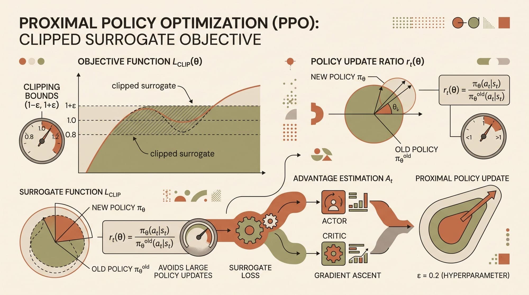
Reinforcement learning from human feedback (RLHF) transformed autoregressive large language models from raw next-token predictors into instruction-following assistants. At the computational center of the foundational RLHF pipelines introduced in InstructGPT (Ouyang et al., 2022) is Proximal Policy Optimization (PPO), formulated by John Schulman, Filip Wolski, Prafulla Dhariwal, Alec Radford, and Oleg Klimov at OpenAI in 2017.

PPO resolved a fundamental instability in policy gradient methods: the destructive impact of large parameter updates on policy behavior. In standard supervised learning, a bad gradient step slightly degrades loss on the current batch but rarely causes permanent divergence. In reinforcement learning, where training data is generated dynamically by the model's own policy, a single destabilizing gradient step can shift policy distributions into degenerate regimes from which recovery is mathematically impossible.

While Trust Region Policy Optimization (TRPO) previously established theoretical convergence guarantees by bounding policy divergence with the Kullback-Leibler (KL) divergence, TRPO relies on second-order optimization, requiring Fisher Information Matrix approximations and conjugate gradient iterations that are computationally intractable for modern billion-parameter LLMs. PPO achieves comparable trust-region stability using a first-order, gradient-clipped surrogate objective that integrates directly with standard stochastic gradient optimizers such as AdamW.

Mathematical Foundations of Policy Gradients and Importance Sampling

In a standard Markov Decision Process (MDP) defined by states $s \in \mathcal{S}$, actions $a \in \mathcal{A}$, transition dynamics $P(s' | s, a)$, and reward function $r(s, a)$, a parameterized policy $\pi_\theta(a | s)$ generates trajectories $\tau = (s_0, a_0, s_1, a_1, \dots, s_T)$.

The expected discounted return under policy $\pi_\theta$ is defined as:

$$J(\theta) = \mathbb{E}_{\tau \sim \pi_\theta} \left[ \sum_{t=0}^T \gamma^t r(s_t, a_t) \right]$$

The standard Policy Gradient Theorem (Sutton et al., 1999) establishes that the analytical gradient of expected return with respect to policy parameters $\theta$ is:

$$\nabla_\theta J(\theta) = \mathbb{E}_{s_t \sim \rho_{\pi_\theta}, a_t \sim \pi_\theta} \left[ \nabla_\theta \log \pi_\theta(a_t | s_t) A^{\pi_\theta}(s_t, a_t) \right]$$

where $\rho_{\pi_\theta}$ is the state distribution and $A^{\pi_\theta}(s_t, a_t) = Q^{\pi_\theta}(s_t, a_t) - V^{\pi_\theta}(s_t)$ represents the advantage function, measuring whether taking action $a_t$ in state $s_t$ performs better or worse than the average action under policy $\pi_\theta$.

This expectation translates into the standard policy gradient objective:

$$L^{PG}(\theta) = \hat{\mathbb{E}}_t \left[ \log \pi_\theta(a_t | s_t) \hat{A}_t \right]$$

The Off-Policy Importance Sampling Formulation

Evaluating $L^{PG}(\theta)$ requires generating fresh rollouts from $\pi_\theta$ after every parameter update. To improve sample efficiency and permit multiple epochs of minibatch updates on a single rollout buffer, PPO applies importance sampling.

If samples $(s_t, a_t)$ are gathered under an older policy $\pi_{\theta_{\text{old}}}$, the expected objective under current parameters $\theta$ is rewritten as:

$$L^{CPI}(\theta) = \hat{\mathbb{E}}_t \left[ \frac{\pi_\theta(a_t | s_t)}{\pi_{\theta_{\text{old}}}(a_t | s_t)} \hat{A}_t \right] = \hat{\mathbb{E}}_t \left[ r_t(\theta) \hat{A}_t \right]$$

where $r_t(\theta)$ denotes the probability ratio:

$$r_t(\theta) = \frac{\pi_\theta(a_t | s_t)}{\pi_{\theta_{\text{old}}}(a_t | s_t)}$$

At the start of an update iteration where $\theta = \theta_{\text{old}}$, the ratio evaluates to $r_t(\theta_{\text{old}}) = 1$. The gradient of $L^{CPI}(\theta)$ at $\theta = \theta_{\text{old}}$ is identical to the standard policy gradient:

$$\left. \nabla_\theta L^{CPI}(\theta) \right|_{\theta = \theta_{\text{old}}} = \left. \hat{\mathbb{E}}_t \left[ \frac{\nabla_\theta \pi_\theta(a_t | s_t)}{\pi_{\theta_{\text{old}}}(a_t | s_t)} \hat{A}_t \right] \right|_{\theta = \theta_{\text{old}}} = \hat{\mathbb{E}}_t \left[ \nabla_\theta \log \pi_\theta(a_t | s_t) \hat{A}_t \right] = \nabla_\theta L^{PG}(\theta_{\text{old}})$$

However, optimizing $L^{CPI}(\theta)$ without constraints across multiple gradient steps causes rapid divergence. If an action yields a positive advantage estimate $\hat{A}_t > 0$, maximizing $r_t(\theta)\hat{A}_t$ pushes $r_t(\theta) \to \infty$, causing large, uncontrolled shifts in policy probabilities. Conversely, when $\hat{A}_t < 0$, $r_t(\theta)$ can be driven to zero, causing policy collapse.

The Clipped Surrogate Objective ($L^{CLIP}$)

To eliminate excessive policy divergence without solving constrained second-order equations, PPO introduces the clipped surrogate objective:

$$L^{CLIP}(\theta) = \hat{\mathbb{E}}_t \left[ \min\left(r_t(\theta)\hat{A}_t, \, \text{clip}(r_t(\theta), 1-\epsilon, 1+\epsilon)\hat{A}_t\right) \right]$$

where $\epsilon$ is a hyperparameter defining the trust region width, typically set to $\epsilon \in [0.1, 0.2]$.

The clipping function bounds the probability ratio within the interval $[1-\epsilon, 1+\epsilon]$:

$$\text{clip}(r_t(\theta), 1-\epsilon, 1+\epsilon) = \begin{cases} 1 - \epsilon & \text{if } r_t(\theta) < 1 - \epsilon \\ r_t(\theta) & \text{if } 1 - \epsilon \le r_t(\theta) \le 1 + \epsilon \\ 1 + \epsilon & \text{if } r_t(\theta) > 1 + \epsilon \end{cases}$$

Four Operating Regimes of the Clipped Objective

The interaction between the sign of advantage $\hat{A}_t$ and the probability ratio $r_t(\theta)$ yields four distinct optimization behaviors:

1. Positive Advantage ($\hat{A}_t > 0$), Below Upper Bound ($r_t(\theta) \le 1+\epsilon$):

The action performed better than baseline expectation. The objective evaluates to $r_t(\theta)\hat{A}_t$. Gradients increase the probability of taking this action in state $s_t$.

1. Positive Advantage ($\hat{A}_t > 0$), Exceeding Upper Bound ($r_t(\theta) > 1+\epsilon$):

The policy has already substantially increased the action probability relative to $\pi_{\theta_{\text{old}}}$. The term $\text{clip}(r_t(\theta), 1-\epsilon, 1+\epsilon)\hat{A}_t$ evaluates to $(1+\epsilon)\hat{A}_t$. Because $(1+\epsilon)\hat{A}_t < r_t(\theta)\hat{A}_t$, the $\min$ operator selects the clipped value: $$\min(r_t(\theta)\hat{A}_t, (1+\epsilon)\hat{A}_t) = (1+\epsilon)\hat{A}_t$$ Because $(1+\epsilon)\hat{A}_t$ is constant with respect to $\theta$, the gradient evaluates to zero ($\nabla_\theta L^{CLIP} = 0$). This cuts off further parameter updates, preventing the optimizer from excessively biasing the policy toward a single advantageous sample.

1. Negative Advantage ($\hat{A}_t < 0$), Above Lower Bound ($r_t(\theta) \ge 1-\epsilon$):

The action performed worse than expected. The objective evaluates to $r_t(\theta)\hat{A}_t$. Gradients decrease the probability of this action.

1. Negative Advantage ($\hat{A}_t < 0$), Below Lower Bound ($r_t(\theta) < 1-\epsilon$):

When $\hat{A}_t < 0$, multiplying by the scalar flips the inequality: $(1-\epsilon)\hat{A}_t > r_t(\theta)\hat{A}_t$. The $\min$ operator selects the unclipped value: $$\min(r_t(\theta)\hat{A}_t, (1-\epsilon)\hat{A}_t) = r_t(\theta)\hat{A}_t$$ Gradients remain active, allowing the policy to continue driving down the probability of an undesirable action if an earlier gradient step made it more likely. Conversely, if $r_t(\theta) > 1+\epsilon$ while $\hat{A}_t < 0$, the clipped term $(1+\epsilon)\hat{A}_t$ is smaller than $r_t(\theta)\hat{A}_t$, capping the penalty and preventing unbounded gradient spikes.

The Pessimistic Lower Bound

Taking the minimum between the unclipped surrogate objective and the clipped surrogate objective guarantees that $L^{CLIP}(\theta)$ forms a conservative, pessimistic lower bound on the true unconstrained importance-sampled objective:

$$L^{CLIP}(\theta) \le L^{CPI}(\theta) = r_t(\theta)\hat{A}_t$$

By maximizing this lower bound, PPO ensures that improvements in the objective translate to true improvements in expected return, eliminating the risk of catastrophic policy drift during multi-epoch minibatch updates.

Generalized Advantage Estimation (GAE)

Accurate estimation of the advantage term $\hat{A}_t$ is necessary for stable policy optimization. Standard Monte Carlo returns exhibit high variance, while single-step Temporal Difference (TD) targets introduce high bias when value function approximations are imperfect.

PPO pairs its clipped surrogate loss with Generalized Advantage Estimation (GAE) (Schulman et al., 2015). GAE defines an exponentially-weighted average of $k$-step advantage estimators controlled by decay parameter $\lambda \in [0, 1]$ and discount factor $\gamma \in [0, 1]$.

Let the 1-step TD residual (temporal difference error) at time $t$ be:

$$\delta_t^V = r_t + \gamma V_\phi(s_{t+1}) - V_\phi(s_t)$$

where $V_\phi(s)$ is a parameterized critic (value network). The generalized advantage estimator $\hat{A}_t^{\text{GAE}(\gamma, \lambda)}$ is formulated as:

$$\hat{A}_t^{\text{GAE}(\gamma, \lambda)} = \sum_{l=0}^\infty (\gamma \lambda)^l \delta_{t+l}^V = \delta_t^V + (\gamma \lambda) \hat{A}_{t+1}^{\text{GAE}(\gamma, \lambda)}$$

The parameter $\lambda$ navigates the bias-variance trade-off:

• When $\lambda = 0$, $\hat{A}_t^{\text{GAE}} = \delta_t^V = r_t + \gamma V_\phi(s_{t+1}) - V_\phi(s_t)$, reducing to a low-variance, high-bias 1-step TD advantage.
• When $\lambda = 1$, $\hat{A}_t^{\text{GAE}} = \sum_{l=0}^\infty \gamma^l r_{t+l} - V_\phi(s_t)$, reducing to an unbiased, high-variance Monte Carlo advantage estimator.

In production LLM alignment, empirical benchmarks typically set $\gamma = 1.0$ (because sequence lengths are finite) and $\lambda \in [0.95, 0.99]$. Advantage values are then normalized across the batch to have zero mean and unit variance ($\hat{A}_t \leftarrow \frac{\hat{A}_t - \mu_A}{\sigma_A + 10^{-8}}$) before calculating $L^{CLIP}(\theta)$.

Complete Actor-Critic Objective and Value Function Clipping

In actor-critic architectures where the policy network $\pi_\theta$ (actor) and value network $V_\phi$ (critic) are trained jointly, the complete optimization objective balances the clipped policy loss, the value function squared error loss, and an entropy regularization term:

$$\mathcal{L}^{PPO}(\theta, \phi) = \hat{\mathbb{E}}_t \left<a href="s_t"> L^{CLIP}(\theta) - c_1 L^{VF}(\phi) + c_2 S[\pi_\theta</a> \right]$$

where $c_1, c_2 > 0$ are hyperparameter coefficients and $S\pi_\theta$ represents the Shannon entropy of the policy distribution, encouraging exploration:

$$S<a href="s_t">\pi_\theta</a> = -\sum_{a \in \mathcal{A}} \pi_\theta(a | s_t) \log \pi_\theta(a | s_t)$$

Clipped Value Loss ($L^{VF}$)

Similar to policy updates, value function optimization can suffer from instability if updates to $V_\phi(s_t)$ diverge excessively from the old value predictions $V_{\phi_{\text{old}}}(s_t)$. To prevent large value updates from corrupting advantage calculations in subsequent iterations, PPO clips the value function:

$$L^{VF}(\phi) = \frac{1}{2} \hat{\mathbb{E}}_t \left[ \max\left( \left(V_\phi(s_t) - V_t^{\text{targ}}\right)^2, \, \left(V_{\phi_{\text{old}}}(s_t) + \text{clip}(V_\phi(s_t) - V_{\phi_{\text{old}}}(s_t), -\epsilon_v, \epsilon_v) - V_t^{\text{targ}}\right)^2 \right) \right]$$

where $V_t^{\text{targ}} = \hat{A}_t^{\text{GAE}} + V_{\phi_{\text{old}}}(s_t)$ is the empirical return target. The $\max$ operator enforces a pessimistic bound on value regression, penalizing parameter updates that over-correct toward noisy return targets.

PPO in LLM Alignment: The 4-Model RLHF Pipeline

Applying PPO to autoregressive language models requires formalizing text generation as a discrete-time Markov Decision Process:

• State $s_t$: The prompt tokens $x$ concatenated with all generated tokens up to step $t$: $s_t = (x, y_1, y_2, \dots, y_{t-1})$.
• Action $a_t$: The discrete token selected from vocabulary $\mathcal{V}$ at step $t$: $a_t = y_t \in \mathcal{V}$.
• Transition Dynamics: Deterministic append operation: $s_{t+1} = (s_t, y_t)$.
• Terminal State: Occurs when the model generates the end-of-sequence token [EOS] or reaches maximum context length $T$.

Executing PPO on LLMs requires orchestrating four distinct neural models simultaneously:

                  ┌───────────────────────────────┐
                  │    Prompt Dataset (x ~ D)     │
                  └──────────────┬────────────────┘
                                 │
                 ┌───────────────┴───────────────┐
                 ▼                               ▼
       ┌──────────────────┐            ┌──────────────────┐
       │   Actor Model    │            │ Reference Model  │
       │  π_θ (Trainable) │            │ π_ref (Frozen)   │
       └────────┬─────────┘            └────────┬─────────┘
                │ Rollout y ~ π_θ               │ Logits π_ref(y|x)
                ├───────────────────────────────┤
                │ Compute Per-Token KL Penalty  │
                │ r_t_pen = r_t - β * KL_div    │
                └───────────────┬───────────────┘
                                │
                 ┌──────────────┴───────────────┐
                 ▼                              ▼
       ┌──────────────────┐           ┌──────────────────┐
       │   Reward Model   │           │   Critic Model   │
       │   r_ψ (Frozen)   │           │  V_φ (Trainable) │
       └────────┬─────────┘           └────────┬─────────┘
                │ Scalar Reward R(x, y)        │ Baseline Value V(s_t)
                └───────────────┬──────────────┘
                                │
                                ▼
                 ┌──────────────────────────────┐
                 │    GAE Advantage & Return    │
                 │      Â_t = GAE(γ, λ)         │
                 └──────────────┬───────────────┘
                                │
                 ┌──────────────┴───────────────┐
                 ▼                              ▼
       ┌──────────────────┐           ┌──────────────────┐
       │ PPO-Clip Update  │           │ Value MSE Update │
       │   ∇_θ L_CLIP     │           │    ∇_φ L_VF      │
       └──────────────────┘           └──────────────────┘

1. Actor Model ($\pi_\theta$): The primary causal language model being aligned, initialized from the Supervised Fine-Tuning (SFT) checkpoint.
2. Reference Model ($\pi_{\text{ref}}$): A frozen duplicate of the initial SFT model. It evaluates log-probabilities on the generated sequence to prevent the actor from drifting into gibberish or reward-hacking modes.
3. Reward Model ($r_\psi$): A frozen transformer trained on paired human preference data via the Bradley-Terry preference model ($P(y_w \succ y_l | x) = \sigma(r_\psi(x, y_w) - r_\psi(x, y_l))$). It emits a scalar score $r_\psi(x, y)$ evaluating the full completion.
4. Critic Model ($V_\phi$): A trainable value model, typically initialized from the reward model with an output linear regression head, that predicts the expected return from any token prefix $s_t$.

Per-Token Reward Transformation and KL Regularization

A naive implementation of RLHF where scalar reward $r_\psi(x, y)$ is applied only at the final token [EOS] suffers from extreme reward sparsity. Furthermore, unconstrained maximization of $r_\psi(x, y)$ leads to severe reward model overoptimization (Goodhart's Law), where the policy exploits flaws in $r_\psi$ to generate degenerate text.

To enforce linguistic coherence, PPO penalizes the token-level reward at each step $t$ using the analytical Kullback-Leibler divergence between actor policy $\pi_\theta$ and reference policy $\pi_{\text{ref}}$:

$$r_t^{\text{pen}}(s_t, y_t) = \begin{cases} -\beta \log \left( \frac{\pi_\theta(y_t | s_t)}{\pi_{\text{ref}}(y_t | s_t)} \right) & \text{if } t < T \\ r_\psi(x, y) - \beta \log \left( \frac{\pi_\theta(y_t | s_t)}{\pi_{\text{ref}}(y_t | s_t)} \right) & \text{if } t = T \end{cases}$$

where $\beta > 0$ controls the strength of the KL penalty. The term $\log \frac{\pi_\theta(y_t | s_t)}{\pi_{\text{ref}}(y_t | s_t)}$ represents the exact point-wise log-likelihood ratio. If the actor assigns a significantly higher probability to a token than the reference policy did, this ratio is positive, deducting from the reward at step $t$.

The Generalized Advantage Estimator is computed over this penalized reward sequence $r_1^{\text{pen}}, \dots, r_T^{\text{pen}}$ using critic values $V_\phi(s_t)$, providing token-level credit assignment throughout the entire generation.

Comparative Analysis: PPO vs TRPO vs DPO vs GRPO

The evolution of post-training alignment algorithms reflects a continuous effort to balance optimization stability, mathematical rigor, and GPU memory utilization.

• TRPO (2015): Second-order constrained optimization enforcing hard trust regions ($\mathbb{E}[D_{KL}] \le \delta$) via conjugate gradient; requires 3 models (Actor, Critic, Reference); high computational overhead from Hessian-vector products.
• PPO (2017): First-order optimization with soft clipped surrogate objectives ($r_t(\theta) \in [1-\epsilon, 1+\epsilon]$); full 4-model architecture (Actor, Critic, Reference, Reward); high stability via normalized GAE and value clipping.
• DPO (2023): Offline closed-form likelihood loss with implicit reward KL regularization; 2-model architecture (Actor, Reference); eliminates critic and reward models; cannot perform active exploration or programmatic verification.
• GRPO (2024): First-order online RL with group relative baselines; 2-model architecture (Actor, Reference); eliminates critic network by computing baseline returns across group rollouts.

Algorithmic Trade-Offs

While Direct Preference Optimization (DPO) (Rafailov et al., 2023) analytically eliminates the reward model and critic by expressing ground-truth preference probabilities directly through policy ratios, DPO operates purely offline on static preference datasets. It cannot explore out-of-distribution trajectories or leverage automated programmatic verification (such as unit test execution or mathematical rule checks).

Group Relative Policy Optimization (GRPO) (Shao et al., 2024), utilized in models like DeepSeek-R1, maintains PPO's online exploration capabilities while eliminating the critic network $V_\phi$. GRPO generates $G$ outputs per prompt $\{y_1, y_2, \dots, y_G\}$ and computes baseline returns as the group mean $\frac{1}{G}\sum r_i$, slashing memory requirements by roughly 50% compared to standard 4-model PPO.

Nonetheless, PPO remains the foundational algorithm for dense, multi-step environments and continuous actor-critic reinforcement learning, providing the mathematical bedrock for modern reinforcement learning in autonomous systems and foundation model post-training.

Sources

• Schulman, J., Wolski, F., Dhariwal, P., Radford, A., & Klimov, O. (2017). Proximal Policy Optimization Algorithms. arXiv:1707.06347. https://arxiv.org/abs/1707.06347
• Schulman, J., Moritz, P., Levine, S., Jordan, M., & Abbeel, P. (2015). High-Dimensional Continuous Control Using Generalized Advantage Estimation. arXiv:1506.02438. https://arxiv.org/abs/1506.02438
• Schulman, J., Levine, S., Moritz, P., Jordan, M., & Abbeel, P. (2015). Trust Region Policy Optimization. arXiv:1502.05477. https://arxiv.org/abs/1502.05477
• Ouyang, L., Wu, J., Jiang, X., Almeida, D., Wainwright, C. L., Mishkin, P., ... & Lowe, R. (2022). Training language models to follow instructions with human feedback. arXiv:2203.02155. https://arxiv.org/abs/2203.02155
• Rafailov, R., Sharma, A., Mitchell, E., Ermon, S., Manning, C. D., & Finn, C. (2023). Direct Preference Optimization: Your Language Model is Secretly a Reward Model. arXiv:2305.18290. https://arxiv.org/abs/2305.18290
• Shao, Z., Wang, P., Zhu, Q., Xu, R., Song, J., Bi, X., ... & Guo, D. (2024). DeepSeekMath: Pushing the Limits of Mathematical Reasoning in Open Language Models. arXiv:2402.03300. https://arxiv.org/abs/2402.03300
• Sutton, R. S., McAllester, D., Singh, S., & Mansour, Y. (1999). Policy Gradient Methods for Reinforcement Learning with Function Approximation. Advances in Neural Information Processing Systems (NeurIPS 1999). https://proceedings.neurips.cc/paper_files/paper/1999/file/464d8283e3e4f0a7ab6cd076779430f8-Paper.pdf
• Bradley, R. A., & Terry, M. E. (1952). Rank Analysis of Incomplete Block Designs: I. The Method of Paired Comparisons. Biometrika, 39(3/4), 324-345. https://www.jstor.org/stable/2334029