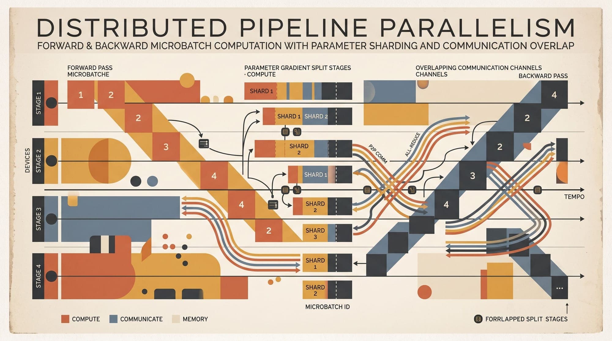
Pipeline Parallelism in Production LLM Training: Comparing 1F1B, Interleaved 1F1B, Zero-Bubble, and DualPipe Schedules

Training modern large language models spanning hundreds of billions of parameters requires distributing model layers across multiple compute nodes. While Tensor Parallelism (TP) partitions individual matrix multiplications across GPUs within a single node, its reliance on high-frequency, all-reduce communications limits its practical scaling to the high-bandwidth domain of NVLink (typically 8 GPUs per node). To scale models beyond single-node memory boundaries, distributed training systems rely on Pipeline Parallelism (PP), which partitions the model depth-wise across successive pipeline stages.

The central engineering challenge in pipeline parallelism is the pipeline bubble: worker GPUs remain idle during pipeline warmup and cooldown while waiting for activations or gradients to propagate across sequential stages. Over the past five years, pipeline scheduling has progressed from naive batching to interleaved virtual stages, decoupled gradient passes, and bidirectional communication-computation overlap.

The Pipeline Bubble Formulation

In pipeline parallelism, a model with $L$ layers is partitioned across $p$ pipeline stages, with each stage hosted on an independent GPU or tensor-parallel group. A global batch is subdivided into $m$ microbatches.

In the baseline GPipe schedule introduced by Huang et al. (2019), all $m$ microbatches execute their forward passes sequentially from stage 0 to stage $p-1$, followed by backward passes in reverse order. The total execution time includes idle intervals during which downstream stages wait for forward activations and upstream stages wait for backward gradients.

The ideal computation time without idle bubbles is:

$$T_{ideal} = m \cdot (t_F + t_B)$$

where $t_F$ represents the forward computation time per microbatch on one stage, and $t_B$ represents the backward computation time.

In GPipe, the idle bubble duration per iteration spans $(p - 1) \cdot (t_F + t_B)$. The bubble fraction $F_{bubble}$ is expressed as:

$$F_{bubble} = \frac{(p - 1) \cdot (t_F + t_B)}{m \cdot (t_F + t_B) + (p - 1) \cdot (t_F + t_B)} = \frac{p - 1}{m + p - 1}$$

To reduce $F_{bubble}$ below 10%, engineering teams must set $m \ge 9p$. However, scaling $m$ arbitrarily is constrained by several physical factors:

1. Global Batch Size Limits: The global batch size is $B_{global} = m \cdot b_{micro} \cdot DP$, where $b_{micro}$ is the microbatch size and $DP$ is the data-parallel degree. Expanding $m$ increases $B_{global}$, which can degrade optimization dynamics and validation loss beyond critical batch size thresholds.
2. Activation Memory Explosion: In GPipe, every stage must store activations for all $m$ microbatches until backpropagation completes, causing GPU out-of-memory (OOM) failures on long context windows.

1F1B Scheduling (PipeDream)

To resolve the activation memory scaling of GPipe, Narayanan et al. (2019) introduced the One Forward, One Backward (1F1B) schedule in PipeDream and adapted it for memory-efficient LLM pre-training in Megatron-LM (Narayanan et al., 2021).

Execution Mechanics

Instead of batching all forward passes together, 1F1B divides execution into three distinct phases:

1. Warmup Phase: Stage $k$ executes $p - k - 1$ consecutive forward passes to fill the pipeline.
2. Steady-State Phase: Once the first backward pass is received from the subsequent stage, each stage alternates strictly between executing one backward pass and one forward pass ($1B \to 1F$).
3. Cooldown Phase: After all $m$ forward passes are completed, stages process the remaining $p - k - 1$ backward passes.

Stage 3:       [F0][F1][F2][F3][B0][F4][B1][F5][B2][F6][B3][B4][B5][B6]
Stage 2:    [F0][F1][F2][F3][F4][B0][F5][B1][F6][B2][B3][B4][B5][B6]
Stage 1: [F0][F1][F2][F3][F4][F5][B0][F6][B1][B2][B3][B4][B5][B6]
Stage 0: [F0][F1][F2][F3][F4][F5][F6][B0][B1][B2][B3][B4][B5][B6]
Time  -->

Resource Characteristics

In 1F1B, the maximum number of in-flight microbatches stored in memory on any stage is capped at $p$. Peak activation memory scales with $O(p)$ rather than $O(m)$, allowing training with large microbatch counts without exhausting device high-bandwidth memory (HBM).

However, 1F1B maintains the same bubble overhead as GPipe:

$$T_{bubble}^{1F1B} = (p - 1) \cdot (t_F + t_B)$$

The bubble ratio remains approximately $\frac{p - 1}{m}$.

Interleaved 1F1B (Megatron-LM 1F1B-I)

To reduce the bubble ratio without increasing global batch size, Megatron-LM introduced Interleaved 1F1B (1F1B-I).

Virtual Stage Partitioning

In 1F1B-I, each physical GPU hosts $v$ virtual stages (model chunks) rather than a single contiguous block of layers. For example, with $p = 4$ physical stages and $v = 2$ virtual stages per device:

• Device 0 hosts Chunk 0 (layers 0-3) and Chunk 4 (layers 16-19)
• Device 1 hosts Chunk 1 (layers 4-7) and Chunk 5 (layers 20-23)
• Device 2 hosts Chunk 2 (layers 8-11) and Chunk 6 (layers 24-27)
• Device 3 hosts Chunk 3 (layers 12-15) and Chunk 7 (layers 28-31)

Microbatches cycle through all physical devices twice: forward passes travel Device $0 \to 1 \to 2 \to 3 \to 0 \to 1 \to 2 \to 3$, and backward passes travel in reverse order.

Bubble and Overhead Trade-Offs

Interleaving shortens the pipeline bubble duration by a factor of $v$:

$$T_{bubble}^{1F1B-I} = \frac{(p - 1) \cdot (t_F + t_B)}{v}$$

The corresponding bubble fraction decreases to:

$$F_{bubble}^{1F1B-I} \approx \frac{p - 1}{v \cdot m}$$

This reduction introduces two engineering costs:

1. Communication Volume: Point-to-point (P2P) peer transfers over network interfaces scale up by $v \times$, increasing cross-node InfiniBand traffic.
2. Activation Footprint: Storing activations across multiple virtual chunks increases peak activation memory by $(v - 1) \cdot b_{micro}$ per stage. In production systems, $v$ is typically constrained to 2 or 4.

Zero-Bubble Pipeline Parallelism (ZB-1P, ZB-2P, ZB-V)

While 1F1B and 1F1B-I treat the backward pass as an indivisible block of time $t_B$, Qi et al. (ICLR 2024) demonstrated that backward computation comprises two distinct operations with differing dependency requirements.

Decoupling Activation and Weight Gradients

For a parameterized layer $y = Wx$, computing the backward pass given incoming gradient $\frac{\partial L}{\partial y}$ requires:

1. Activation Gradient ($B_x$ or $B$):

$$\frac{\partial L}{\partial x} = \frac{\partial L}{\partial y} W^T$$ This gradient must be transmitted immediately to the upstream pipeline stage so that earlier layers can continue backpropagation.

1. Parameter/Weight Gradient ($B_W$ or $W$):

$$\frac{\partial L}{\partial W} = \left(\frac{\partial L}{\partial y}\right)^T x$$ This tensor is accumulated locally into the gradient buffer for the optimizer update. No other pipeline stage requires this tensor during the forward-backward iteration.

In standard Transformer layers, the computational cost divides roughly as $t_F \approx t_B \approx t_W$, where $t_B$ (computing $\frac{\partial L}{\partial x}$) represents $1/3$ of total backward computation and $t_W$ (computing $\frac{\partial L}{\partial W}$) represents the remaining $2/3$.

Standard Backward (2/3 total step time):
[------------- Backward Step t_B_total -------------]
[-- Activation Grad B_x (t_B) --][-- Weight Grad B_W (t_W) --]
 ^ Required by Stage k-1          ^ Local accumulation only

ZB-1P and ZB-2P Scheduling

Because $W$ computation does not sit on the critical latency path of backpropagation, Zero-Bubble schedules decouple $B$ and $W$:

• The activation gradient computation ($B$) is executed immediately to keep upstream stages active.
• The parameter gradient computation ($W$) is deferred and scheduled into the idle intervals (bubbles) during warmup, steady state, and cooldown.

In ZB-1P (Zero-Bubble 1-Phase), $W$ kernels are prioritized such that peak activation memory remains identical to standard 1F1B ($p$ microbatches). The resulting bubble duration decreases to:

$$T_{bubble}^{ZB-1P} = (p - 1) \cdot (t_F + t_B - 2t_W)$$

When $t_F \approx t_B \approx t_W$, $T_{bubble}^{ZB-1P}$ approaches zero in steady state.

In ZB-2P, the schedule allows peak activation memory to reach $2p$ microbatches, enabling an optimizer-validated reordering where all pipeline bubbles are filled by deferred $W$ passes. ZB-V combines this decoupling with virtual stage interleaving to achieve zero bubble under equivalent memory bounds.

Bidirectional Overlap: DeepSeek DualPipe

In large-scale Mixture of Experts (MoE) architectures such as DeepSeek-V3 and DeepSeek-R1 (DeepSeek-AI, 2024), inter-node All-to-All communication for routed experts introduces substantial network latency. To eliminate both pipeline idle bubbles and communication overheads, DeepSeek introduced DualPipe, an open-source bidirectional pipeline parallelism schedule (GitHub: deepseek-ai/DualPipe).

Bidirectional Microbatch Streams

DualPipe deploys two symmetrical pipelines running simultaneously in opposite directions on the same physical infrastructure:

• Forward Stream 0: Flows from Stage $0 \to p - 1$
• Forward Stream 1: Flows from Stage $p - 1 \to 0$

Each physical GPU is assigned two symmetric chunks: one from the first half of the model and one from the second half.

DualPipe Physical Mapping (PP = 4):
GPU 0: Chunk 0 (Layers 0..15)   & Chunk 7 (Layers 96..111)
GPU 1: Chunk 1 (Layers 16..31)  & Chunk 6 (Layers 80..95)
GPU 2: Chunk 2 (Layers 32..47)  & Chunk 5 (Layers 64..79)
GPU 3: Chunk 3 (Layers 48..63)  & Chunk 4 (Layers 64..79)

Overlapped Forward-Backward Kernels ($F\&B$)

DualPipe integrates the $B/W$ gradient splitting of Zero-Bubble with kernel-level computation-communication overlap. During steady state, DualPipe executes combined $F\&B$ instructions:

1. As a forward chunk executes its dense matrix multiplications, it simultaneously drives the asynchronous non-blocking All-to-All communication of MoE dispatch for a backward chunk.
2. The backward pass activation gradient ($B$) and weight gradient ($W$) are interleaved directly between forward activations.

DualPipe Computation-Communication Overlap:
[---------------- Computation Track ----------------]
[ Forward GEMM (Chunk A) ][ Backward GEMM (Chunk B) ]
[---------------- Communication Track --------------]
[ P2P Recv (Chunk B)     ][ MoE All-to-All (Chunk A) ]
<------- Synchronous Execution over Dual Streams ------>

The bubble duration in DualPipe drops to:

$$T_{bubble}^{DualPipe} = \left(\frac{p}{2} - 1\right) \cdot (t_{F\&B} + t_B - 3t_W)$$

where $t_{F\&B}$ is the execution time of the fused forward-backward overlap kernel.

Architectural Comparison and Systems Economics

The choice of pipeline parallel schedule determines the trade-off between memory allocation, network pressure, and GPU Model FLOPs Utilization (MFU).

| Feature / Metric | 1F1B (PipeDream) | Interleaved 1F1B | Zero-Bubble (ZB-1P) | DeepSeek DualPipe | | :--- | :--- | :--- | :--- | :--- | | Bubble Time | $(p - 1)(t_F + t_B)$ | $\frac{p - 1}{v}(t_F + t_B)$ | $(p - 1)(t_F + t_B - 2t_W)$ | $\left(\frac{p}{2} - 1\right)(t_{F\&B} + t_B - 3t_W)$ | | Typical Bubble Fraction | $15\% - 30\%$ | $5\% - 12\%$ | $2\% - 6\%$ | $< 1.5\%$ | | Peak Activation Memory | $p \cdot b_{micro}$ | $(p + v - 1) \cdot b_{micro}$ | $p \cdot b_{micro}$ | $(p + 1) \cdot b_{micro}$ | | Model Parameter Copies | $1\times$ | $1\times$ | $1\times$ | $2\times$ (Shared stages per GPU) | | P2P Network Volume | Baseline ($1\times$) | $v\times$ Baseline | Baseline ($1\times$) | $2\times$ Baseline | | MoE All-to-All Overlap | None | Limited | None | Full asynchronous overlap | | Kernel Complexity | Standard PyTorch | Standard PyTorch | Custom autograd engine | Custom dual-stream overlap |

Implementation Considerations in Production Clusters

When deploying advanced pipeline schedules in production clusters running Megatron-Core, DeepSpeed, or custom frameworks, several systems considerations apply:

1. Autograd Hook Splitting: Standard PyTorch torch.autograd.backward() bundles tensor and parameter gradient passes into a single execution graph. Implementing Zero-Bubble or DualPipe requires registering manual tensor hooks or custom C++/CUDA backward kernels that emit $\frac{\partial L}{\partial x}$ and return immediately, queuing $\frac{\partial L}{\partial W}$ onto a secondary worker queue.
2. CUDA Stream Synchronization: DualPipe requires multi-stream management (typically separate compute, P2P send, P2P receive, and All-to-All collective streams). Unbalanced microbatch execution times can introduce intra-device synchronization bubbles if GPU SM occupancy is saturated by GEMM kernels during non-blocking communication passes.
3. Memory Budget Allocation: In MoE pre-training, parameter memory is dominated by routed experts. Because DualPipe assigns two distinct layer chunks to each physical device, the model parameter memory per GPU doubles unless weights are sharded via ZeRO-style distributed optimizers across data-parallel groups.

Sources

• PipeDream: Fast and Efficient Pipeline Parallel DNN Training (Narayanan et al., SOSP 2019 / arXiv:1906.00707)
• GPipe: Efficient Training of Giant Neural Networks using Pipeline Parallelism (Huang et al., NeurIPS 2019 / arXiv:1811.06965)
• Efficient Large-Scale Language Model Training on GPU Clusters Using Megatron-LM (Narayanan et al., SC 2021 / arXiv:2104.04473)
• Zero Bubble Pipeline Parallelism (Qi et al., ICLR 2024 / arXiv:2401.10241)
• DeepSeek-V3 Technical Report (DeepSeek-AI, 2024 / arXiv:2412.19437)
• DeepSeek DualPipe Implementation (GitHub: deepseek-ai/DualPipe)