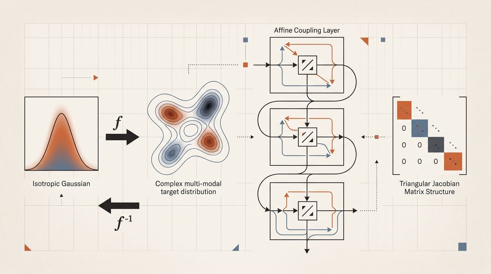
Normalizing Flows and Real NVP: How Invertible Neural Networks and Triangular Jacobians Compute Exact Log-Likelihoods

Generative modeling in deep learning revolves around a fundamental question: how can a neural network learn to transform a simple, analytically tractable probability distribution into a complex, high-dimensional empirical data distribution?

Over the past decade, four primary generative modeling paradigms have emerged to address this challenge:

1. Generative Adversarial Networks (GANs) optimize an implicit minimax objective, producing sharp samples in a single forward pass but failing to provide explicit density estimation or deterministic latent encodings.
2. Variational Autoencoders (VAEs) optimize an evidence lower bound (ELBO) on the data log-likelihood via stochastic approximate posteriors, which yields tractable training but introduces blurry samples due to imperfect posterior approximation and variational gaps.
3. Diffusion and Score-Based Models reverse a progressive noise corruption process via score matching or stochastic differential equations, achieving high sample fidelity at the cost of dozens to hundreds of sequential denoising steps.
4. Normalizing Flows formulate generative modeling through exact, invertible, and differentiable mappings (diffeomorphisms). By leveraging the multivariate change-of-variables theorem, normalizing flows compute exact data log-likelihoods, perform bidirectional single-pass mapping between data and latent spaces, and eliminate both variational bounds and adversarial instabilities.

This article examines the mathematical mechanics and architectural innovations that make normalizing flows possible, focusing on triangular Jacobian structures, affine coupling layers in Real NVP, invertible 1x1 convolutions in Glow, and continuous-time formulations that bridge discrete flows and modern flow matching.

1. The Change of Variables Theorem and the Determinant Bottleneck

At the core of normalizing flows is the probability density transformation under invertible mappings, formalized by the multivariate change-of-variables theorem.

Mathematical Formulation

Let $z \in \mathbb{R}^D$ denote a continuous random variable drawn from a base probability distribution $p_Z(z)$ with an analytically tractable density, such as an isotropic standard Gaussian:

$$p_Z(z) = \mathcal{N}(z; 0, I) = \frac{1}{(2\pi)^{D/2}} \exp\left(-\frac{1}{2} \|z\|_2^2\right)$$

Let $f_\theta: \mathbb{R}^D \rightarrow \mathbb{R}^D$ be a bijective, continuously differentiable function parameterized by neural network weights $\theta$, with a well-defined inverse $g_\theta = f_\theta^{-1}$ such that $z = g_\theta(x) = f_\theta^{-1}(x)$.

When a random vector $z$ is transformed into $x = f_\theta(z)$, conservation of probability mass over an infinitesimal volume element requires:

$$p_X(x) \cdot |dx| = p_Z(z) \cdot |dz|$$

Substituting $z = f_\theta^{-1}(x)$ and relating differential volume elements via the Jacobian matrix $J_{f_\theta^{-1}}(x) = \frac{\partial f_\theta^{-1}(x)}{\partial x}$:

$$p_X(x) = p_Z(f_\theta^{-1}(x)) \cdot \left| \det \left( \frac{\partial f_\theta^{-1}(x)}{\partial x} \right) \right|$$

By the inverse function theorem, the Jacobian of the inverse mapping is the matrix inverse of the forward Jacobian: $\frac{\partial f_\theta^{-1}(x)}{\partial x} = \left(\frac{\partial f_\theta(z)}{\partial z}\right)^{-1}$. Because $\det(A^{-1}) = (\det A)^{-1}$, the density of $x$ can equivalently be expressed in terms of the forward transformation $f_\theta$:

$$p_X(x) = p_Z(f_\theta^{-1}(x)) \cdot \left| \det \left( \frac{\partial f_\theta(z)}{\partial z} \right) \right|^{-1}$$

Taking the natural logarithm yields the exact log-likelihood training objective for a single data point $x$:

$$\log p_X(x) = \log p_Z(f_\theta^{-1}(x)) - \log \left| \det J_{f_\theta}(f_\theta^{-1}(x)) \right|$$

   Data Space X                     Latent Space Z
   (Complex, Multi-modal)           (Simple Isotropic Gaussian)
   
        [ x ]  ------------------------>  [ z = f⁻¹(x) ]
          │          Inference Mode               │
          │                                       │
          │         Exact Likelihood:             │
          │     log p(x) = log p(z) + log|det J|   │
          │                                       │
        [ x = f(z) ]  <------------------------  [ z ]
                     Generation Mode

Compositional Flow Sequences

A single transformation $f_\theta$ is rarely expressive enough to map a standard Gaussian to complex multi-modal image or audio distributions. However, bijections are closed under functional composition. A normalizing flow chains $K$ successive invertible transformations:

$$x = f_K \circ f_{K-1} \circ \dots \circ f_1(z_0), \quad z_0 \sim p_Z(z_0)$$

Setting intermediate representations $z_k = f_k(z_{k-1})$ with $z_K = x$, the inverse path evaluates sequentially:

$$z_{k-1} = f_k^{-1}(z_k)$$

By the chain rule of differentiation, the total Jacobian factorizes into the matrix product of intermediate Jacobians:

$$J_f(z_0) = \prod_{k=1}^K J_{f_k}(z_{k-1})$$

Because the determinant of a matrix product equals the product of individual determinants ($\det(AB) = \det(A)\det(B)$), the total log-determinant decomposes into a straightforward sum over the $K$ flow layers:

$$\log p_X(x) = \log p_Z(z_0) - \sum_{k=1}^K \log \left| \det J_{f_k}(z_{k-1}) \right|$$

The $O(D^3)$ Determinant Bottleneck

Evaluating and training normalizing flows via maximum likelihood requires optimizing $\mathbb{E}_{x \sim p_{data}} [-\log p_X(x)]$. This requires computing two operations efficiently:

1. Inverting the forward mapping: $z = f_\theta^{-1}(x)$ to evaluate $\log p_Z(z)$.
2. Computing the log-determinant of the Jacobian: $\log |\det J_{f_\theta}(z)|$.

For an arbitrary unstructured non-linear transformation $f_\theta: \mathbb{R}^D \rightarrow \mathbb{R}^D$, computing the Jacobian matrix requires $D$ vector-Jacobian products, and evaluating its determinant requires Gaussian elimination or LU decomposition, which scales with $O(D^3)$ arithmetic complexity.

For high-dimensional signals (for example, a $256 \times 256 \times 3$ image has $D = 196,608$), an $O(D^3)$ operation requires approximately $7.6 \times 10^{15}$ floating-point operations per sample, making general unconstrained neural architectures computationally intractable for density estimation.

The core engineering breakthrough of normalizing flows lies in designing constrained neural architectures whose Jacobian matrices exhibit special algebraic structures: specifically, triangular matrices, whose determinants evaluate in linear $O(D)$ time.

2. NICE: Additive Coupling Layers and Volume Preservation

In 2014, Laurent Dinh, David Krueger, and Yoshua Bengio introduced NICE (Non-linear Independent Components Estimation) (arXiv:1410.8516), establishing the foundational coupling layer architecture that circumvented the $O(D^3)$ determinant bottleneck.

Additive Coupling Architecture

To achieve an easily computable Jacobian determinant while maintaining high non-linear expressivity, NICE partitions the input vector $z \in \mathbb{R}^D$ into two disjoint subspaces $z_{1:d}$ and $z_{d+1:D}$, where $d < D$ (typically $d = \lfloor D/2 \rfloor$).

The forward additive coupling transformation is defined as:

$$\begin{aligned} x_{1:d} &= z_{1:d} \\ x_{d+1:D} &= z_{d+1:D} + m(z_{1:d}) \end{aligned}$$

Here, $m: \mathbb{R}^d \rightarrow \mathbb{R}^{D-d}$ is an arbitrary neural network (such as a multi-layer perceptron or deep convolutional network).

   Input Vector z = [ z_{1:d} , z_{d+1:D} ]
                          │           │
           ┌──────────────┴─────┐     │
           │                    │     │
           │  Identity Path     │     │
           │                    ▼     │
           │                 [ m(·) ] │
           │                    │     │
           │                    ▼     ▼
           │                   (+) <──┘  (Additive Shift)
           │                    │
           ▼                    ▼
   Output Vector x = [ x_{1:d} , x_{d+1:D} ]

Analytic Inversion and Triangular Jacobian

The additive coupling architecture possesses two critical properties:

1. Exact, Unconstrained Inversion: The inverse transformation can be written in closed form without inverting the neural network $m(\cdot)$:

$$\begin{aligned} z_{1:d} &= x_{1:d} \\ z_{d+1:D} &= x_{d+1:D} - m(x_{1:d}) \end{aligned}$$ Because $x_{1:d} = z_{1:d}$, the exact same forward pass through $m(\cdot)$ computes the subtraction term during inversion. Consequently, $m(\cdot)$ does not need to be bijective, invertible, or restricted in layer depth, activation choice, or width.

1. Unit Triangular Jacobian: The Jacobian matrix of the forward transformation exhibits a block-triangular structure:

$$J = \frac{\partial x}{\partial z} = \begin{bmatrix} I_d & 0 \\ \frac{\partial m(z_{1:d})}{\partial z_{1:d}} & I_{D-d} \end{bmatrix}$$ The determinant of a block triangular matrix is the product of the determinants of its diagonal blocks: $$\det J = \det(I_d) \cdot \det(I_{D-d}) = 1 \cdot 1 = 1$$ Therefore: $$\log |\det J| = \log(1) = 0$$

Volume Preservation and Diagonal Scaling

Because $\det J = 1$, additive coupling layers are strictly volume preserving: they can shift and warp distributions in space, but they cannot locally expand or compress probability mass.

To allow the model to adjust variance across dimensions, NICE introduces a diagonal scaling layer as the final transformation of the network:

$$x_i = s_i \cdot z_i, \quad s_i > 0$$

The Jacobian of this diagonal scaling layer is a diagonal matrix $\text{diag}(s_1, \dots, s_D)$, whose log-determinant evaluates as:

$$\log |\det J_{scale}| = \sum_{i=1}^D \log s_i$$

While NICE proved that neural networks could compute exact log-likelihoods in linear time, volume-preserving flows struggle with high-dimensional distributions whose intrinsic dimensionality varies widely across manifold neighborhoods.

3. Real NVP: Affine Coupling Layers and Multi-Scale Architectures

In 2016, Laurent Dinh, Jascha Sohl-Dickstein, and Samy Bengio introduced Real NVP (Real-valued Non-Volume Preserving) (arXiv:1605.08803), extending coupling mechanisms to general non-volume-preserving affine transformations and introducing multi-scale multi-channel topologies.

Affine Coupling Mechanism

Real NVP replaces additive shifts with element-wise scale and translation operations. Given partition $z_{1:d}$ and $z_{d+1:D}$:

$$\begin{aligned} x_{1:d} &= z_{1:d} \\ x_{d+1:D} &= z_{d+1:D} \odot \exp(s(z_{1:d})) + t(z_{1:d}) \end{aligned}$$

where:

• $s: \mathbb{R}^d \rightarrow \mathbb{R}^{D-d}$ is a scale network (typically with tanh or bounded activations to prevent numerical explosion).
• $t: \mathbb{R}^d \rightarrow \mathbb{R}^{D-d}$ is a translation network.
• $\odot$ denotes Hadamard (element-wise) multiplication.

Forward and Inverse Dynamics

The inverse mapping of an affine coupling layer requires only element-wise subtraction and division:

$$\begin{aligned} z_{1:d} &= x_{1:d} \\ z_{d+1:D} &= (x_{d+1:D} - t(x_{1:d})) \odot \exp(-s(x_{1:d})) \end{aligned}$$

As in NICE, the neural networks $s(\cdot)$ and $t(\cdot)$ are evaluated exclusively in the forward direction during both generation ($z \to x$) and density estimation / inference ($x \to z$). They can consist of arbitrary Residual Network (ResNet) blocks with batch normalization, dilated convolutions, and non-monotonic activations.

Jacobian Evaluation in $O(D)$

The Jacobian matrix of the affine coupling layer is lower triangular:

$$J = \begin{bmatrix} I_d & 0 \\ \frac{\partial x_{d+1:D}}{\partial z_{1:d}} & \text{diag}(\exp(s(z_{1:d}))) \end{bmatrix}$$

Because the determinant of any triangular matrix is simply the product of its diagonal elements, the non-diagonal partial derivative block $\frac{\partial x_{d+1:D}}{\partial z_{1:d}}$ does not need to be computed or stored:

$$\det J = \prod_{j=1}^{D-d} \exp(s(z_{1:d})_j) = \exp\left( \sum_{j=1}^{D-d} s(z_{1:d})_j \right)$$

Taking the logarithm yields the exact log-determinant:

$$\log |\det J| = \sum_{j=1}^{D-d} s(z_{1:d})_j$$

This reduces the computational cost of the Jacobian log-determinant from $O(D^3)$ to $O(D)$, matching the asymptotic cost of a single forward pass.

Spatial Partitioning and Multi-Scale Topologies

To process high-dimensional spatial data (such as 2D images), Real NVP introduced two spatial masking patterns and a hierarchical multi-scale architecture:

   Checkerboard Masking Pattern         Channel Masking Pattern (Post-Squeeze)
   
        ┌───┬───┬───┬───┐                     ┌───────────────┐
        │ 1 │ 0 │ 1 │ 0 │                     │  Channel 1:d  │ (Identity)
        ├───┼───┼───┼───┤                     ├───────────────┤
        │ 0 │ 1 │ 0 │ 1 │                     │               │
        ├───┼───┼───┼───┤                     │ Channel d+1:D │ (Transformed)
        │ 1 │ 0 │ 1 │ 0 │                     │               │
        ├───┼───┼───┼───┤                     └───────────────┘
        │ 0 │ 1 │ 0 │ 1 │
        └───┴───┴───┴───┘

1. Spatial Checkerboard Masking: Alternates masked and active pixels in a 2D grid across spatial dimensions $(H, W)$.
2. Squeeze Operation and Channel Masking: A deterministic tensor transformation reshapes a tensor of shape $(H, W, C)$ into $(H/2, W/2, 4C)$ by dividing spatial $2 \times 2$ neighborhoods into 4 sub-channels, followed by channel-wise partitioning ($1:2C$ and $2C+1:4C$).
3. Multi-Scale Latent Factoring: After several coupling layers at a given spatial scale, half of the channel dimensions are factored out directly to the Gaussian latent loss:

$$z^{(i)} \sim \mathcal{N}(0, I)$$ The remaining channels continue through subsequent flow blocks at lower spatial resolutions. This reduces intermediate memory requirements by $50\%$ per scale step and enforces a coarse-to-fine hierarchical representation where early layers model high-frequency textures and deeper layers capture global layout.

4. Glow: Invertible 1x1 Convolutions and ActNorm

While Real NVP demonstrated impressive density estimation and image generation capabilities, it relied on fixed, hand-crafted channel permutations (reversing channel order between coupling layers) to ensure that all dimensions interact across successive flow steps.

In 2018, Durk Kingma and Prafulla Dhariwal introduced Glow (Generative Flow with Invertible 1x1 Convolutions) (arXiv:1807.03039), modernizing flow architectures with learnable channel mixing and data-dependent normalization.

       ┌───────────────────────────────────────┐
       │             Step of Flow              │
       │                                       │
       │    [ Input Tensor: (H x W x C) ]      │
       │                  │                    │
       │                  ▼                    │
       │       [ Activation Normalization ]    │
       │                  │                    │
       │                  ▼                    │
       │      [ Invertible 1x1 Conv (W) ]      │
       │                  │                    │
       │                  ▼                    │
       │       [ Affine Coupling Layer ]       │
       │                  │                    │
       └──────────────────┼────────────────────┘
                          ▼

Invertible 1x1 Convolutions

Glow replaces fixed channel permutations with a general linear transformation across channel dimensions:

$$y_{h, w, :} = z_{h, w, :} W$$

where $z \in \mathbb{R}^{H \times W \times C}$ and $W \in \mathbb{R}^{C \times C}$ is a learnable square weight matrix initialized as a random orthogonal matrix ($\det W = \pm 1$).

For an input with spatial dimensions $H \times W$, the Jacobian matrix of this transformation is a block-diagonal matrix composed of $H \cdot W$ identical blocks of $W$. The log-determinant evaluates as:

$$\log \left| \det \left(\frac{\partial y}{\partial z}\right) \right| = H \cdot W \cdot \log |\det W|$$

LU Decomposition Parameterization

Computing $\det W$ directly takes $O(C^3)$ operations. To accelerate both sampling and density evaluation, Glow parameterizes $W$ using the LU decomposition:

$$W = P L (U + \text{diag}(s))$$

where:

• $P \in \mathbb{R}^{C \times C}$ is a fixed permutation matrix (selected at initialization via PLU decomposition and kept constant).
• $L \in \mathbb{R}^{C \times C}$ is a lower triangular matrix with ones on the diagonal.
• $U \in \mathbb{R}^{C \times C}$ is an upper triangular matrix with zeros on the diagonal.
• $s \in \mathbb{R}^C$ is a learnable parameter vector representing the diagonal elements of the upper triangular matrix.

Because $\det(P) \in \{-1, 1\}$, $\det(L) = 1$, and the determinant of an upper triangular matrix is the product of its diagonal elements:

$$\log |\det W| = \sum_{i=1}^C \log |s_i|$$

This reduces the cost of computing the log-determinant during training from $O(C^3)$ to $O(C)$, while computing the matrix inverse $W^{-1} = (U + \text{diag}(s))^{-1} L^{-1} P^{-1}$ requires only fast triangular back-substitution.

Activation Normalization (ActNorm)

Deep normalizing flows are sensitive to initialization and internal covariate shift. Standard batch normalization introduces stochasticity across batch dimensions and requires tracking running statistics, which can introduce discrepancies between training and inference.

Glow introduces ActNorm (Activation Normalization), which applies an affine transformation with learnable scale and bias vectors per channel:

$$y_{h, w, c} = s_c \cdot (x_{h, w, c} + b_c)$$

• Data-Dependent Initialization: On the first forward pass (minibatch 0), $b_c$ is initialized to $-\mu_c$ (minibatch mean) and $s_c$ is initialized to $\frac{1}{\sigma_c + \epsilon}$ (minibatch standard deviation), setting initial activations to zero mean and unit variance.
• Subsequent Optimization: After initialization, $s_c$ and $b_c$ are treated as independent trainable parameters optimized via gradient descent.
• Log-Determinant:

$$\log |\det J_{\text{ActNorm}}| = H \cdot W \cdot \sum_{c=1}^C \log |s_c|$$

5. Continuous Normalizing Flows and FFJORD

While discrete normalizing flows chain discrete transformation layers, Continuous Normalizing Flows (CNFs) formulate flow trajectories via ordinary differential equations (ODEs), bridging normalizing flows with dynamical systems.

The Continuous Change of Variables

Introduced by Ricky T. Q. Chen et al. in Neural Ordinary Differential Equations (arXiv:1806.07366), a continuous normalizing flow defines the state evolution $z(t)$ from $t_0$ to $t_1$ via an ODE parameterized by a neural network dynamics function $f(z(t), t; \theta)$:

$$\frac{dz(t)}{dt} = f(z(t), t; \theta)$$

Integrating from $t_0$ to $t_1$ gives the forward transformation:

$$z(t_1) = z(t_0) + \int_{t_0}^{t_1} f(z(t), t; \theta) dt$$

Under continuous dynamics, the change in log probability density satisfies the instantaneous change of variables formula:

$$\frac{\partial \log p(z(t))}{\partial t} = -\text{Tr}\left( \frac{\partial f(z(t), t; \theta)}{\partial z(t)} \right)$$

Integrating over time yields the total change in log-likelihood:

$$\log p(z(t_1)) = \log p(z(t_0)) - \int_{t_0}^{t_1} \text{Tr}\left( J_f(z(t), t) \right) dt$$

The key mathematical shift: instead of evaluating a matrix determinant $\det(J)$, continuous flows require evaluating the trace of the Jacobian matrix $\text{Tr}(J) = \sum_{i} \frac{\partial f_i}{\partial z_i}$.

   Discrete Flows (Real NVP / Glow)        Continuous Normalizing Flows (FFJORD)
   
        z_0 ──f_1──> z_1 ──f_2──> z_2            z(t_0) ═════════════════════════> z(t_1)
                                                       dz/dt = f(z(t), t; θ)
   • Matrix Determinant: log|det J|          • Matrix Trace: Tr(∂f/∂z)
   • Requires Triangular Structure           • Free-Form Neural Architectures
   • Discrete Step Errors                    • Adaptive Step-Size ODE Solvers

FFJORD and the Hutchinson Trace Estimator

Computing the exact trace of an unconstrained Jacobian still requires $D$ vector-Jacobian products. In 2018, Will Grathwohl et al. introduced FFJORD (Free-form Jacobian of Reversible Dynamics) (arXiv:1810.01367), applying the Hutchinson trace estimator:

$$\text{Tr}(A) = \mathbb{E}_{p(\epsilon)} \left[ \epsilon^T A \epsilon \right]$$

where $\epsilon \in \mathbb{R}^D$ is a random noise vector with zero mean and identity covariance ($\mathbb{E}[\epsilon] = 0$, $\text{Cov}(\epsilon) = I$), typically sampled from a standard Gaussian or Rademacher distribution ($\epsilon_i \in \{-1, +1\}$).

Applying this to the continuous flow objective:

$$\text{Tr}\left( \frac{\partial f}{\partial z} \right) = \mathbb{E}_{p(\epsilon)} \left[ \epsilon^T \left(\frac{\partial f}{\partial z}\right) \epsilon \right]$$

The inner product $\left(\frac{\partial f}{\partial z}\right) \epsilon$ is a single vector-Jacobian product (VJP), computable in a single backward autodiff pass via reverse-mode automatic differentiation in $O(D)$ time.

FFJORD eliminated the need for triangular Jacobian restrictions, allowing continuous flows to employ unconstrained neural architectures (such as standard MLPs, Convnets, and Transformers), which laid the theoretical groundwork for modern Flow Matching (Lipman et al., 2022).

6. Architectural and Performance Comparison

The following table summarizes the mathematical, computational, and operational trade-offs between Normalizing Flows and alternative deep generative modeling paradigms:

| Generative Paradigm | Density Evaluation | Sampling Mechanism | Inversion / Latent Mapping | Jacobian / Constraint Mechanism | Primary Bottleneck | | :--- | :--- | :--- | :--- | :--- | :--- | | GANs (Goodfellow et al.) | Implicit (None) | Single forward pass ($O(1)$) | Non-invertible (Requires optimization) | None (Adversarial discriminator) | Training instability, mode collapse | | VAEs (Kingma & Welling) | Approximate (ELBO lower bound) | Single forward pass ($O(1)$) | Approximate ($q_\phi(z \mid x)$ posterior) | None (Variational divergence regularizer) | Variational gap, blurry reconstructions | | Diffusion / DDPM (Sohl-Dickstein / Ho) | Intractable (ELBO / ODE likelihood) | Iterative SDE/ODE ($N \approx 20\text{--}1000$ steps) | Approximate stochastic backward path | Score matching / Denoising objective | High sampling latency | | Real NVP / Glow (Dinh / Kingma) | Exact ($\log p(x)$ computable) | Single forward pass ($O(1)$) | Exact deterministic bijection ($z = f^{-1}(x)$) | Block-triangular coupling, invertible 1x1 convs | High parameter count, dimension preservation ($z \in \mathbb{R}^D$) | | Continuous Flows / FFJORD (Chen / Grathwohl) | Exact (Via ODE integration) | Adaptive ODE solver integration | Exact (Reverse-time ODE integration) | Hutchinson trace estimator ($\text{Tr}(J)$ via VJP) | Variable ODE integration time during training/inference | | Flow Matching (Lipman et al.) | Exact (Via probability flow ODE) | Fast ODE integration ($N \approx 10\text{--}50$ steps) | Exact (Deterministic ODE reversal) | Optimal Transport regression without simulation | Moderate sampling steps vs. discrete flows |

7. Practical Implementation: Minimal 2D Affine Coupling Flow

To demonstrate the core mechanics of Real NVP, the following clean PyTorch implementation builds an invertible affine coupling layer and stacks multiple blocks to learn a 2D two-moons distribution:

import torch
import torch.nn as nn
import torch.distributions as dist

class AffineCouplingLayer(nn.Module):
    """
    Real NVP Affine Coupling Layer.
    Splits input into (z1, z2), transforms z2 using scale/shift nets conditioned on z1.
    """
    def __init__(self, dim, hidden_dim=64, mask_even=True):
        super().__init__()
        self.dim = dim
        self.mask_even = mask_even
        
        # Partition dimension
        self.d = dim // 2
        in_features = self.d
        out_features = dim - self.d
        
        # Scale and translation networks (arbitrary MLPs)
        self.net_s = nn.Sequential(
            nn.Linear(in_features, hidden_dim),
            nn.GELU(),
            nn.Linear(hidden_dim, hidden_dim),
            nn.GELU(),
            nn.Linear(hidden_dim, out_features),
            nn.Tanh()  # Bound scale factors to stabilize training
        )
        self.net_t = nn.Sequential(
            nn.Linear(in_features, hidden_dim),
            nn.GELU(),
            nn.Linear(hidden_dim, hidden_dim),
            nn.GELU(),
            nn.Linear(hidden_dim, out_features)
        )
        
    def _split(self, x):
        if self.mask_even:
            return x[:, :self.d], x[:, self.d:]
        else:
            return x[:, self.d:], x[:, :self.d]

    def _join(self, x1, x2):
        if self.mask_even:
            return torch.cat([x1, x2], dim=-1)
        else:
            return torch.cat([x2, x1], dim=-1)

    def forward(self, z):
        """Forward mapping: z -> x (Generation direction)"""
        z1, z2 = self._split(z)
        s = self.net_s(z1)
        t = self.net_t(z1)
        
        x1 = z1
        x2 = z2 * torch.exp(s) + t
        x = self._join(x1, x2)
        
        # Log determinant is sum of scale factors
        log_det = torch.sum(s, dim=-1)
        return x, log_det

    def inverse(self, x):
        """Inverse mapping: x -> z (Inference / Density Estimation direction)"""
        x1, x2 = self._split(x)
        s = self.net_s(x1)
        t = self.net_t(x1)
        
        z1 = x1
        z2 = (x2 - t) * torch.exp(-s)
        z = self._join(z1, z2)
        
        # Inverse log determinant is negative sum of scale factors
        log_det = -torch.sum(s, dim=-1)
        return z, log_det

class RealNVP2D(nn.Module):
    """
    Stacked Real NVP Normalizing Flow for 2D density estimation.
    """
    def __init__(self, num_layers=6, hidden_dim=64):
        super().__init__()
        self.layers = nn.ModuleList([
            AffineCouplingLayer(dim=2, hidden_dim=hidden_dim, mask_even=(i % 2 == 0))
            for i in range(num_layers)
        ])
        # Standard 2D isotropic Gaussian base distribution
        self.register_buffer("base_mean", torch.zeros(2))
        self.register_buffer("base_cov", torch.eye(2))

    @property
    def base_distribution(self):
        return dist.MultivariateNormal(self.base_mean, self.base_cov)

    def forward(self, z):
        """Sampling: z ~ N(0, I) -> x"""
        log_det_sum = torch.zeros(z.shape[0], device=z.device)
        x = z
        for layer in self.layers:
            x, log_det = layer.forward(x)
            log_det_sum += log_det
        return x, log_det_sum

    def inverse(self, x):
        """Inference & Density: x -> z, computing exact log p(x)"""
        log_det_sum = torch.zeros(x.shape[0], device=x.device)
        z = x
        for layer in reversed(self.layers):
            z, log_det = layer.inverse(z)
            log_det_sum += log_det
            
        # log p(x) = log p_Z(z) + sum(log |det J_inverse|)
        log_pz = self.base_distribution.log_prob(z)
        log_px = log_pz + log_det_sum
        return z, log_px

Summary and Current Role in AI

Normalizing flows represent one of the most mathematically rigorous frameworks in deep generative modeling. By exploiting structured triangular Jacobians in affine coupling layers, architectures like Real NVP and Glow demonstrated that neural networks can evaluate exact, unconstrained log-likelihoods and execute single-pass bidirectional sampling in $O(D)$ time without variational approximations.

While discrete normalizing flows face architectural constraints (such as preserving exact dimensionality $z \in \mathbb{R}^D$ and requiring substantial parameter depth for complex image synthesis), their mathematical principles remain vital across contemporary machine learning:

1. Exact Likelihood Estimation & Out-of-Distribution Detection: Benchmarking density estimators and modeling high-energy physics particle collision kinematics.
2. Molecular Conformation and Protein Modeling: Generating physically consistent 3D atomic coordinates subject to SE(3) equivariance constraints.
3. High-Fidelity Audio Synthesis: Powering real-time, low-latency waveform generators such as WaveGlow.
4. Foundations of Modern Flow Matching: Supplying the theoretical and differential geometry frameworks that underpin modern continuous flow matching in frontier vision, speech, and video models.

Sources

• Dinh, L., Krueger, D., & Bengio, Y. (2014). NICE: Non-linear Independent Components Estimation. arXiv:1410.8516
• Dinh, L., Sohl-Dickstein, J., & Bengio, S. (2016). Density estimation using Real NVP. arXiv:1605.08803
• Kingma, D. P., & Dhariwal, P. (2018). Glow: Generative Flow with Invertible 1x1 Convolutions. arXiv:1807.03039
• Rezende, D. J., & Mohamed, S. (2015). Variational Inference with Normalizing Flows. arXiv:1505.05770
• Chen, R. T. Q., Rubanova, Y., Bettencourt, J., & Duvenaud, D. (2018). Neural Ordinary Differential Equations. arXiv:1806.07366
• Grathwohl, W., Chen, R. T. Q., Bettencourt, J., Sutskever, I., & Duvenaud, D. (2018). FFJORD: Free-form Jacobian of Reversible Dynamics for Scalable Invertible Generative Modeling. arXiv:1810.01367
• Papamakarios, G., Nalisnick, E., Rezende, D. J., Mohamed, S., & Lakshminarayanan, B. (2021). Normalizing Flows for Probabilistic Modeling and Inference. Journal of Machine Learning Research (JMLR) / arXiv:1912.02762
• Lipman, Y., Chen, R. T. Q., Ben-Hamu, H., Nicklas, M., & Le, M. (2022). Flow Matching for Generative Modeling. arXiv:2210.02747