Non-Contrastive Representation Learning: How Barlow Twins and VICReg Prevent Feature Collapse via Redundancy Reduction

Self-supervised representation learning provides the foundation for modern foundation models across computer vision, audio, and multimodal systems. By training deep neural networks to produce compact vector embeddings without human annotations, self-supervised pre-training enables models to capture rich semantic structures directly from raw data.

Historically, the dominant approach to self-supervised learning was contrastive learning, popularized by architectures such as SimCLR (Chen et al., 2020) and MoCo (He et al., 2020). Contrastive methods optimize the InfoNCE objective: they pull representations of augmented views of the same sample together while actively pushing representations of different samples apart.

While effective, contrastive learning imposes severe practical constraints. To prevent representation collapse, contrastive frameworks require hundreds or thousands of negative pairs per batch. This dependency forces practitioners to maintain massive mini-batch sizes (typically 2,048 to 4,096 samples), construct complex memory banks, or run momentum encoders. Furthermore, negative sampling introduces false-negative bias, where semantically similar samples from different sources are incorrectly penalized for having aligned representations.

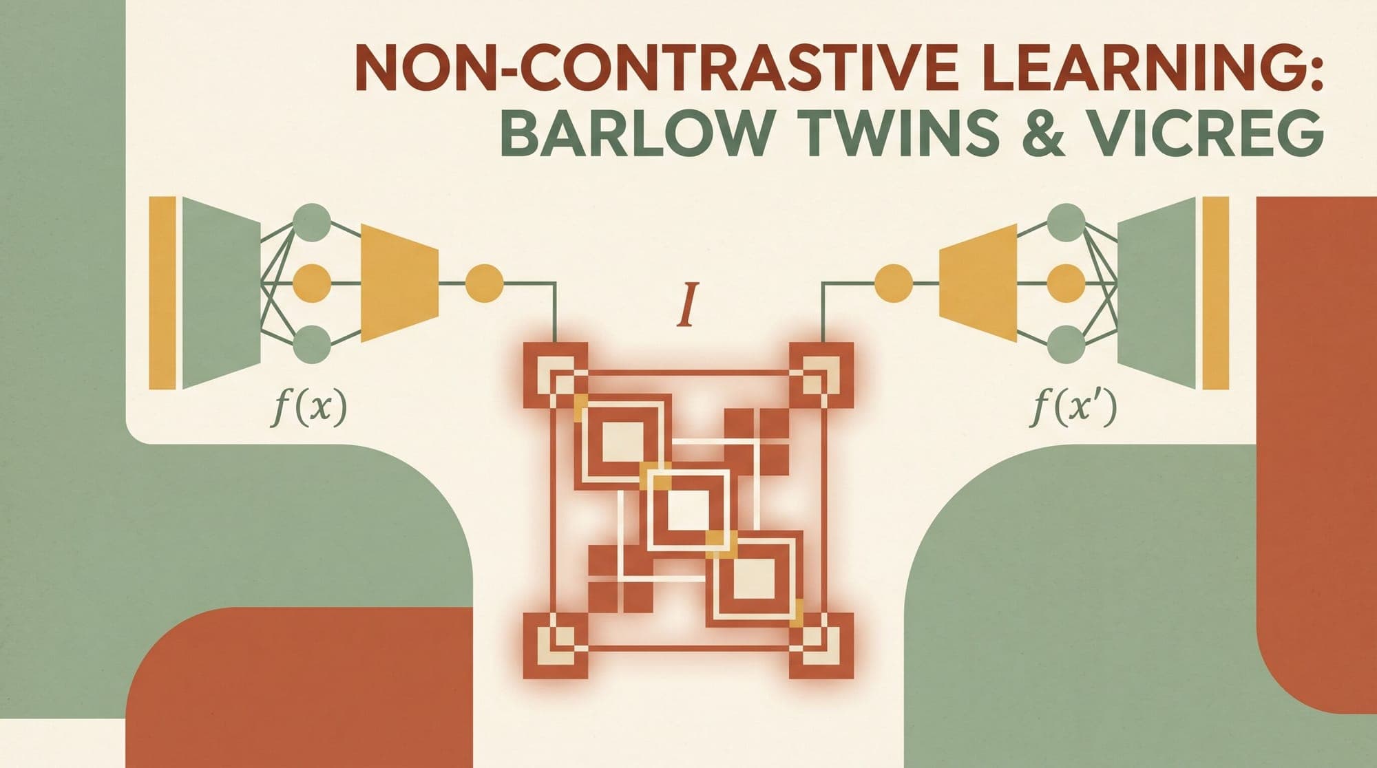
Non-contrastive self-supervised learning eliminates negative pairs entirely. Architectures such as Barlow Twins (Zbontar et al., 2021) and VICReg (Bardes et al., 2022) prevent representation collapse through statistical regularization across embedding dimensions. By operating directly on the cross-correlation matrix or decomposing the objective into explicit variance, invariance, and covariance terms, these methods enable stable representation learning on standard batch sizes without negative sampling or architectural asymmetries.

The Mechanics of Representation Collapse

To understand why non-contrastive objectives are necessary, consider a naive Siamese network trained solely to minimize the distance between two augmented views of the same input:

$$\mathcal{L}_{\text{naive}} = \frac{1}{N} \sum_{i=1}^N \|z_i^A - z_i^B\|_2^2$$

where $z_i^A = g_\theta(f_\theta(x_i^A))$ and $z_i^B = g_\theta(f_\theta(x_i^B))$ represent the projector embeddings of two augmented views $x_i^A$ and $x_i^B$ of sample $x_i$.

Without negative pairs or regularization constraints, minimizing this objective leads to two catastrophic collapse failure modes:

1. Complete (Constant) Collapse: The network maps all inputs to an identical constant vector $z_i = \mathbf{c}$ for all $x_i$. In this state, $\|z_i^A - z_i^B\|_2 = 0$, achieving a global loss of zero while discarding all input information.
2. Dimensional (Informational) Collapse: The network avoids a constant vector, but the output representations span only a tiny lower-dimensional subspace or hyperplane within the embedding space. When dimensional collapse occurs, the covariance matrix of the embeddings exhibits near-zero rank. The model utilizes only a fraction of its available capacity, and individual feature dimensions become entirely redundant and collinear.

Heuristic Approaches to Collapse Prevention

Before explicit non-contrastive regularization, empirical methods prevented collapse through architectural asymmetries and optimization dynamics:

• BYOL (Grill et al., 2020): Introduces an online network and a target network. The target network parameters are updated as an exponential moving average (EMA) of the online network parameters. An additional asymmetric predictor MLP is placed on the online branch, and gradients are stopped along the target branch ($\text{stop\_gradient}$).
• SimSiam (Chen & He, 2021): Demonstrates that Siamese networks can learn without negative pairs or momentum encoders, relying strictly on an asymmetric prediction MLP combined with a $\text{stop\_gradient}$ operation on one branch.

While BYOL and SimSiam avoid complete collapse in practice, their stability depends on precise hyperparameter tuning, batch normalization placement, and optimizer momentum dynamics. They prevent collapse implicitly rather than providing an exact mathematical constraint on representation entropy.

Barlow Twins: Redundancy Reduction via Cross-Correlation

Barlow Twins (Zbontar et al., 2021) introduced a principled objective rooted in neurobiology. The framework adapts the redundancy reduction hypothesis formulated by neuroscientist Horace Barlow in 1961, which posited that sensory processing systems transform raw sensory inputs into neural codes that minimize statistical redundancy among neuronal firing patterns.

The Barlow Twins Architecture and Loss Formulation

The Barlow Twins pipeline processes input images through the following steps:

1. Data Augmentation: An input image $x$ is transformed into two distorted views, $x^A$ and $x^B$, using standard augmentations (random cropping, color jittering, Gaussian blur, and solarization).
2. Feature Extraction and Projection: Both views pass through a shared encoder backbone $f_\theta$ (such as ResNet-50 or a Vision Transformer) to produce representations $y^A$ and $y^B$. These representations pass through a non-linear projector MLP $g_\theta$ with three linear layers, batch normalization, and ReLU activations, yielding embeddings $Z^A, Z^B \in \mathbb{R}^{N \times D}$, where $N$ is batch size and $D$ is embedding dimension.
3. Cross-Correlation Computation: The embeddings are normalized along the batch dimension such that each feature dimension has a mean of zero and unit variance across the batch. The cross-correlation matrix $\mathcal{C} \in \mathbb{R}^{D \times D}$ between the twin outputs is computed as:

$$\mathcal{C}_{ij} = \frac{\sum_{b=1}^N z_{b, i}^A z_{b, j}^B}{\sqrt{\sum_{b=1}^N (z_{b, i}^A)^2} \sqrt{\sum_{b=1}^N (z_{b, j}^B)^2}}$$

The Barlow Twins loss function forces $\mathcal{C}$ toward the identity matrix $\mathbf{I}_D$:

$$\mathcal{L}_{\text{BT}} = \sum_{i=1}^D (1 - \mathcal{C}_{ii})^2 + \lambda \sum_{i=1}^D \sum_{j \neq i}^D \mathcal{C}_{ij}^2$$

where $\lambda$ is a positive weighting hyperparameter (typically set to $5 \times 10^{-3}$).

Decomposing the Barlow Twins Loss

The loss consists of two complementary terms:

• Invariance Term (Diagonal Elements $\mathcal{C}_{ii}$): By forcing $\mathcal{C}_{ii} \to 1$, the network ensures that the $i$-th dimension of $Z^A$ is perfectly correlated with the $i$-th dimension of $Z^B$. This encourages the representations to remain invariant to the applied data distortions.
• Redundancy Reduction Term (Off-Diagonal Elements $\mathcal{C}_{ij}$ for $i \neq j$): By penalizing non-zero cross-correlations $\mathcal{C}_{ij} \to 0$, the network decorrelates the individual feature dimensions. This prevents different output neurons from encoding redundant signals, forcing the model to maximize informational capacity and preventing dimensional collapse.

Because the objective evaluates correlations across the feature dimension $D$ rather than across batch samples $N$, Barlow Twins operates effectively on high-dimensional projector outputs ($D = 8,192$). As $D$ increases, downstream linear evaluation accuracy scales monotonically without overfitting.

VICReg: Variance, Invariance, and Covariance Regularization

While Barlow Twins resolved negative pair dependence, its cross-correlation matrix couples the invariance and decorrelation operations across twin branches. VICReg (Bardes, Ponce, & LeCun, 2022) introduced an explicit tripartite decomposition that isolates the geometric requirements of non-contrastive representation learning into three independent regularization terms: Variance, Invariance, and Covariance.

The Mathematical Formulation of VICReg

Given two batches of projector embeddings $Z^A = [z_1^A, \dots, z_N^A]^T \in \mathbb{R}^{N \times D}$ and $Z^B = [z_1^B, \dots, z_N^B]^T \in \mathbb{R}^{N \times D}$ from two augmented views:

1. Invariance Criterion $s(Z^A, Z^B)$

The invariance term measures the mean squared Euclidean distance between corresponding sample embeddings:

$$s(Z^A, Z^B) = \frac{1}{N} \sum_{i=1}^N \|z_i^A - z_i^B\|_2^2$$

This pulls the representations of two views of the same scene together in latent space.

2. Variance Regularization Criterion $v(Z)$

To prevent complete collapse to a single constant vector, VICReg enforces a hinge loss on the standard deviation of each feature dimension across the batch:

$$v(Z) = \frac{1}{D} \sum_{j=1}^D \max\left(0, \gamma - S(z^j, \epsilon)\right)$$

where $\gamma$ is a target standard deviation threshold (typically $\gamma = 1$), $\epsilon$ is a small numerical stabilizer ($10^{-4}$), and $S(z^j, \epsilon)$ is the empirical regularized standard deviation of dimension $j$:

$$S(z^j, \epsilon) = \sqrt{\frac{1}{N-1} \sum_{i=1}^N \left(z_{i, j} - \bar{z}_j\right)^2 + \epsilon}, \quad \bar{z}_j = \frac{1}{N} \sum_{i=1}^N z_{i, j}$$

If the standard deviation of any embedding dimension falls below $\gamma$, the hinge loss exerts a repelling gradient that forces the representations to spread out along that coordinate axis.

3. Covariance Regularization Criterion $c(Z)$

To prevent dimensional collapse, where features become linearly dependent and span a lower-dimensional subspace, VICReg decorrelates distinct dimensions by minimizing the off-diagonal elements of the sample covariance matrix $C(Z)$:

$$C(Z) = \frac{1}{N-1} \sum_{i=1}^N (z_i - \bar{z})(z_i - \bar{z})^T$$

$$c(Z) = \frac{1}{D} \sum_{i=1}^D \sum_{j \neq i}^D [C(Z)]_{ij}^2$$

Minimizing $c(Z)$ forces the off-diagonal covariance entries to zero, driving $C(Z)$ toward a diagonal matrix. This decorrelates feature dimensions, ensuring that each dimension captures orthogonal, non-redundant information.

The Combined Objective

The total VICReg loss function is a weighted linear combination of the three terms evaluated across both branches:

$$\mathcal{L}_{\text{VICReg}} = \lambda s(Z^A, Z^B) + \mu \left(v(Z^A) + v(Z^B)\right) + \nu \left(c(Z^A) + c(Z^B)\right)$$

In standard ImageNet pre-training configurations, the hyperparameters are set to $\lambda = 25.0$, $\mu = 25.0$, and $\nu = 1.0$.

Architectural Comparison Across Self-Supervised Paradigms

The table below contrasts contrastive, asymmetric, and non-contrastive self-supervised architectures across their operational mechanics, memory profiles, and collapse prevention techniques:

| Architecture | Paradigm | Primary Objective | Collapse Prevention Mechanism | Negative Pairs Required | Batch Size Sensitivity | | :--- | :--- | :--- | :--- | :--- | :--- | | SimCLR (Chen et al., 2020) | Contrastive | InfoNCE Cross-Entropy | Negative sample repulsion in denominator | Yes (thousands per batch) | High (Requires $N \ge 2048$ for peak performance) | | MoCo-v2 (He et al., 2020) | Contrastive | InfoNCE with Memory Queue | Negative sample memory queue + Momentum Encoder | Yes (65,536 queue size) | Low to Medium (Decoupled by memory queue) | | BYOL (Grill et al., 2020) | Asymmetric Bootstrap | Mean Squared Error | Predictor MLP + Momentum Encoder + Stop-Gradient | No | Medium (Relies on batch normalization statistics) | | SimSiam (Chen & He, 2021) | Asymmetric Siamese | Cosine Similarity | Predictor MLP + Stop-Gradient | No | Low to Medium (Prone to collapse without stop-gradient) | | Barlow Twins (Zbontar et al., 2021) | Non-Contrastive | Cross-Correlation Identity Loss | Redundancy reduction on off-diagonal correlation | No | Low (Stable across $N = 128$ to $N = 2048$) | | VICReg (Bardes et al., 2022) | Non-Contrastive | Variance + Invariance + Covariance | Hinge variance loss + Off-diagonal covariance penalty | No | Low (Maintains performance with standard mini-batches) |

Key Optimization and Architectural Insights

Practical implementations of Barlow Twins and VICReg reveal several critical design principles:

1. The Role of High-Dimensional Expansion Projectors

Both Barlow Twins and VICReg utilize an expansion projector MLP $g_\theta$ placed on top of the encoder backbone $f_\theta$. While the backbone output dimension is typically $D_{\text{backbone}} = 2,048$ (for a standard ResNet-50) or $768$ (for ViT-Base), the projector maps embeddings to a higher-dimensional space:

$$D_{\text{projector}} \in [4,096, 8,192]$$

Empirical studies in Zbontar et al. (2021) and Bardes et al. (2022) demonstrate that expanding projector dimensionality allows the covariance and cross-correlation penalties to decorrelate thousands of fine-grained feature combinations. After pre-training completes, the projector MLP is discarded; the frozen backbone representations $y = f_\theta(x)$ are used for downstream classification, object detection, and segmentation tasks.

2. Elimination of Stop-Gradients and Asymmetries

Unlike BYOL and SimSiam, neither Barlow Twins nor VICReg requires asymmetric architectures:

• Both branches share identical weight parameters ($f_\theta$ and $g_\theta$).
• Gradients backpropagate symmetrically through both branches.
• No exponential moving average (EMA) momentum encoder is needed.
• No specialized stop-gradient operations are inserted into the computational graph.

This architectural symmetry simplifies distributed training across multi-node GPU clusters, eliminating synchronization overhead associated with maintaining twin parameter copies.

3. Independence from Memory Banks and False Negatives

Because non-contrastive methods evaluate statistical dispersion across feature dimensions rather than instance-level discrimination across the dataset, they are immune to false negative penalties. In standard contrastive learning, two distinct images containing the same object category (for example, two different golden retrievers) are treated as negative pairs, penalizing the model for learning semantic invariance. Non-contrastive objectives avoid this penalty, leading to cleaner clustering in downstream linear probe evaluations.

Modern Extensions: From Vision to Foundation Architectures

The principles introduced by Barlow Twins and VICReg have expanded across diverse domains:

• Dense Representation Learning (VICRegL): Bardes et al. (2022) extended VICReg to local feature maps (VICRegL), applying variance and covariance penalties simultaneously to global image representations and fine-grained spatial grid locations for object detection and semantic segmentation.
• Joint-Embedding Predictive Architectures (JEPA): Meta's I-JEPA (Assran et al., 2023) and V-JEPA (Bardes et al., 2024) build upon non-contrastive representation principles, predicting missing spatial and temporal representations in latent space rather than pixel space to train self-supervised world models.
• Multimodal and Cross-Modal Alignment: Non-contrastive objectives are increasingly utilized in audio-visual alignment, graph neural networks, and tabular representation pre-training, providing stable gradient dynamics in domains where defining negative pairs is noisy or computationally intractable.

By replacing sample-wise repulsion with coordinate-wise redundancy reduction, non-contrastive self-supervised learning established a scalable mathematical foundation for representation learning without the sample complexity overhead of contrastive pairs.

Sources

• Zbontar, J., Jing, L., Misra, I., LeCun, Y., & Deny, S. (2021). Barlow Twins: Self-Supervised Learning via Redundancy Reduction. Proceedings of the 38th International Conference on Machine Learning (ICML 2021), PMLR 139:12310-12320.
• Bardes, A., Ponce, J., & LeCun, Y. (2022). VICReg: Variance-Invariance-Covariance Regularization for Self-Supervised Learning. International Conference on Learning Representations (ICLR 2022).
• Chen, T., Kornblith, S., Norouzi, M., & Hinton, G. (2020). A Simple Framework for Contrastive Learning of Visual Representations. Proceedings of the 37th International Conference on Machine Learning (ICML 2020), PMLR 119:1597-1607.
• Grill, J. B., Strub, F., Altché, F., Tallec, C., Richemond, P. H., Buchatskaya, E., ... & Valko, M. (2020). Bootstrap Your Own Latent: A New Approach to Self-Supervised Learning. Advances in Neural Information Processing Systems (NeurIPS 2020), 33:21271-21284.
• Chen, X., & He, K. (2021). Exploring Simple Siamese Representation Learning. IEEE/CVF Conference on Computer Vision and Pattern Recognition (CVPR 2021), 15750-15758.
• Assran, M., Duval, Q., Misra, I., Bojanowski, P., Vincent, P., Rabbat, M., LeCun, Y., & Ballas, N. (2023). Self-Supervised Learning from Images with a Joint-Embedding Predictive Architecture. IEEE/CVF Conference on Computer Vision and Pattern Recognition (CVPR 2023), 14471-14480.
• Bardes, A., Ponce, J., & LeCun, Y. (2022). VICRegL: Self-Supervised Learning of Local Visual Features. Advances in Neural Information Processing Systems (NeurIPS 2022), 35:8799-8810.
• Barlow, H. B. (1961). Possible Principles Underlying the Transformation of Sensory Messages. Sensory Communication, 1:217-234.