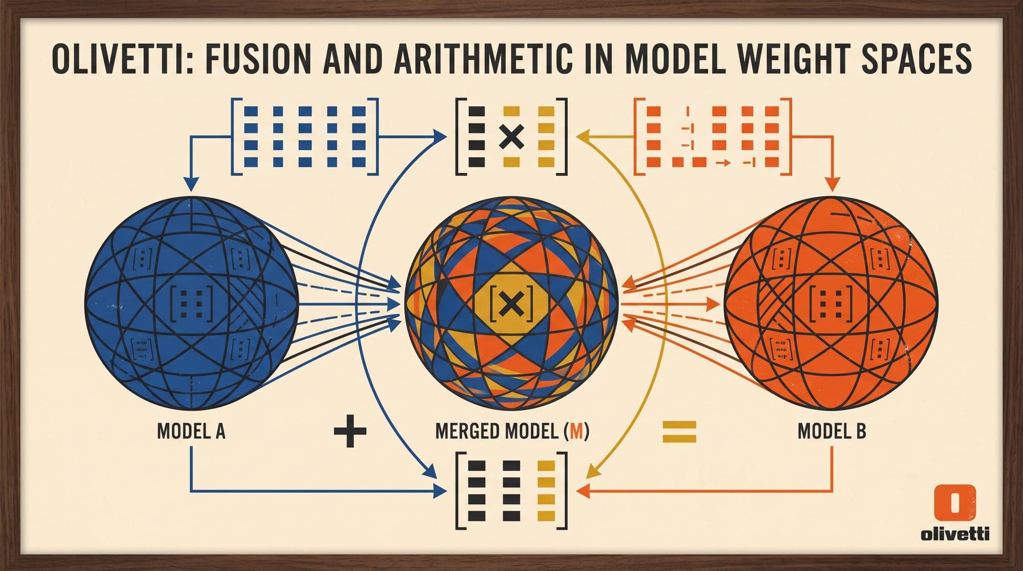
Model Merging in Weight Space: Mathematical Foundations of Task Vectors, TIES-Merging, DARE, and Spherical Linear Interpolation

Training large language models across multiple downstream domains typically requires expensive multi-task supervised fine-tuning (SFT) or sequential continual learning. Both paths present steep practical challenges: multi-task training demands simultaneous access to massive, curated datasets and massive compute budgets, while sequential fine-tuning suffers from catastrophic forgetting.

Model merging has emerged as a data-free, compute-efficient alternative. By combining the parameters of multiple specialized models derived from a shared pre-trained base directly in weight space, practitioners can fuse disparate skills (such as mathematical reasoning, instruction following, and multilingual fluency) into a single checkpoint without additional backpropagation or inference latency overhead.

Understanding how model merging functions requires examining the geometry of neural network loss landscapes, the algebra of task vectors, and the algorithmic strategies designed to resolve high-dimensional parameter interference.

The Geometry of Weight Space and Linear Mode Connectivity

The premise of weight-space merging relies on Linear Mode Connectivity (Frankle et al., 2020). While deep neural network loss surfaces are non-convex, models fine-tuned from the same pre-trained initialization ( $\theta_{\text{pre}}$ ) often reside within the same low-loss basin. Within this basin, linear paths between different fine-tuned solutions do not encounter severe loss barriers.

The simplest approach to model merging is uniform parameter averaging, popularized in Model Soups (Wortsman et al., 2022). Given $M$ fine-tuned checkpoints $\theta_1, \theta_2, \dots, \theta_M$ originating from $\theta_{\text{pre}}$ , the averaged model is defined as:

$\theta_{\text{soup}} = \frac{1}{M} \sum_{i=1}^M \theta_i$

While effective for checkpoints trained on the same task with different hyperparameters or random seeds, uniform averaging fails when merging models fine-tuned on diverse, distinct tasks. Diverse tasks pull parameters in conflicting directions, leading to destructive parameter interference and performance degradation.

Task Vectors and Task Arithmetic

To merge distinct capabilities, Ilharco et al. (2023) introduced the concept of Task Vectors. A task vector $\tau_t$ represents the directional shift in weight space induced by fine-tuning a pre-trained base model $\theta_{\text{pre}}$ on a specific task $t$ :

$\tau_t = \theta_t - \theta_{\text{pre}}$

Because $\tau_t$ isolates the task-specific parameter delta, weight modifications can be treated algebraically:

1. Multi-Task Addition

To synthesize multiple capabilities into a single base model, practitioners compute the linear combination of task vectors scaled by a hyperparameter $\lambda$ :

$\theta_{\text{merged}} = \theta_{\text{pre}} + \lambda \sum_{t=1}^T \tau_t$

2. Task Negation and Unlearning

Task arithmetic enables targeted behavioral steering without retraining. To reduce an undesirable behavior (such as toxicity, hallucination patterns, or memorized sensitive data), the corresponding task vector can be negated:

$\theta_{\text{steered}} = \theta_{\text{target}} - \lambda \tau_{\text{undesirable}}$

3. Analogical Transfer

Task vectors can also transfer properties across domains using vector arithmetic analogies ( $A - B + C \approx D$ ), modifying domain-specific behaviors without direct downstream training data.

Despite its simplicity, naive task addition struggles as the number of tasks $T$ scales, because parameter updates from orthogonal tasks begin to cancel or corrupt one another.

Spherical Linear Interpolation (SLERP)

When merging two model checkpoints, standard linear interpolation (LERP), $\theta(t) = (1-t)\theta_0 + t\theta_1$ , suffers from high-dimensional geometric collapse. In high-dimensional spaces, linear interpolation between two vectors of similar magnitude pulls the intermediate vector closer to the origin:

$\|\theta(t)\| < \min(\|\theta_0\|, \|\theta_1\|) \quad \text{for } 0 < t < 1$

This norm shrinking alters parameter scale distributions, disrupting layer normalization and attention scaling in transformers.

Spherical Linear Interpolation (SLERP) (Shoemake, 1985; White, 2016) resolves this issue by interpolating along the great circle arc on a multi-dimensional hypersphere, preserving vector magnitude and constant angular velocity.

Linear Interpolation (LERP):
θ₀ ───────•───────> θ₁  (interpolated vector cuts through the sphere; norm shrinks)

Spherical Linear Interpolation (SLERP):
   ╭──────•──────╮
θ₀ ╵             ╵ θ₁  (interpolated vector follows constant radius along arc)

The mathematical formulation proceeds as follows:

Normalize both parameter vectors to unit vectors:

$\hat{\theta}_0 = \frac{\theta_0}{\|\theta_0\|}, \quad \hat{\theta}_1 = \frac{\theta_1}{\|\theta_1\|}$

Compute the angle $\Omega$ between the vectors using the inner product:

$\cos \Omega = \hat{\theta}_0 \cdot \hat{\theta}_1, \quad \Omega = \arccos(\hat{\theta}_0 \cdot \hat{\theta}_1)$

Compute the interpolated vector along the arc for interpolation parameter $t \in [0, 1]$ :

$\text{SLERP}(\theta_0, \theta_1; t) = \frac{\sin((1-t)\Omega)}{\sin \Omega} \theta_0 + \frac{\sin(t\Omega)}{\sin \Omega} \theta_1$

When $\sin \Omega \to 0$ (collinear vectors), the formulation gracefully degenerates to standard linear interpolation. SLERP is applied layer-by-layer across weight tensors, preserving scale properties across transformer blocks.

Resolving Interference: TIES-Merging

While SLERP handles pairwise model fusion, multi-task merging requires resolving parameter conflicts across three or more models. In TIES-Merging (Yadav et al., NeurIPS 2023), the authors identified two primary sources of degradation during multi-task vector summation:

Redundant Parameter Interference: Fine-tuning introduces millions of small, noisy parameter changes that do not contribute significantly to task performance but accumulate destructively when summed across models.
Sign Disagreement Interference: Different tasks often require contradictory updates to the same parameter ( ${\text{sign}}(\tau_{a, j}) \neq {\text{sign}}(\tau_{b, j})$ ). Summing them directly results in mutual cancellation, destroying both capabilities.

To resolve these failure modes, TIES-Merging introduces a three-stage algorithm: TRIM, ELECT SIGN, and DISJOINT MERGE.

Stage 1: Trim (Quantile Pruning)

For each task vector $\tau_t \in \mathbb{R}^d$ , retain only the top $k\%$ (typically $k \in [10, 30]$ ) parameter changes with the largest absolute magnitude, setting the remaining $(100-k)\%$ to zero:

$\hat{\tau}_{t, j} = \begin{cases} \tau_{t, j} & \text{if } |\tau_{t, j}| \ge \text{Quantile}_{1 - \frac{k}{100}}(|\tau_t|) \\ 0 & \text{otherwise} \end{cases}$

This step strips away redundant parameter noise while preserving task-critical delta features.

Stage 2: Elect Sign (Consensus Direction)

For each parameter index $j$ , resolve directional conflicts by calculating the total signed magnitude mass across all trimmed task vectors:

$\gamma_j = \text{sign}\left(\sum_{t=1}^T \hat{\tau}_{t, j}\right)$

The vector $\gamma \in \{-1, +1\}^d$ represents the majority consensus update direction for each parameter in weight space.

Stage 3: Disjoint Merge (Selective Averaging)

For each parameter index $j$ , compute the merged delta by averaging only the task updates whose signs agree with the elected sign $\gamma_j$ :

$S_j = \{t \in \{1, \dots, T\} : \text{sign}(\hat{\tau}_{t, j}) = \gamma_j \text{ and } \hat{\tau}_{t, j} \neq 0\}$

$\tau_{\text{merged}, j} = \begin{cases} \frac{1}{|S_j|} \sum_{t \in S_j} \hat{\tau}_{t, j} & \text{if } |S_j| > 0 \\ 0 & \text{otherwise} \end{cases}$

The final model weights are reconstructed by adding the scaled merged delta to the pre-trained base:

$\theta_{\text{merged}} = \theta_{\text{pre}} + \lambda \tau_{\text{merged}}$

By discarding opposing gradients rather than allowing them to cancel out consensus directions, TIES-Merging retains task accuracy across diverse domains.

DARE: Drop And Rescale

Building upon parameter sparsity, Yu et al. (ICML 2024) introduced DARE (Drop And REscale). The authors observed an extreme redundancy property in supervised fine-tuning: between 90% and 99% of delta parameters in homologous models can be eliminated entirely without substantial performance degradation, provided the surviving weights are appropriately rescaled.

DARE models parameter pruning as a stochastic dropout process followed by an expectation-preserving scaling step.

Mathematical Formulation

Given task vector $\tau_t$ , DARE generates a random binary Bernoulli mask $m_t \sim \text{Bernoulli}(p)$ , where $p \in [0, 1)$ represents the drop rate (typically $p \ge 0.90$ ). The sparsified, rescaled task vector $\tilde{\tau}_t$ is computed as:

$\tilde{\tau}_t = \frac{1}{1 - p} \left((1 - m_t) \odot \tau_t\right)$

Where $\odot$ denotes element-wise multiplication.

Expectation Invariance Proof

Because parameter masking is independent across coordinates, the expected value of the sparsified parameter equals the original parameter delta:

$\mathbb{E}[\tilde{\tau}_{t, j}] = \frac{1}{1 - p} \mathbb{E}[1 - m_{t, j}] \cdot \tau_{t, j} = \frac{1}{1 - p} (1 - p) \cdot \tau_{t, j} = \tau_{t, j}$

By scaling surviving weights by $\frac{1}{1-p}$ , DARE preserves the aggregate activation magnitude across transformer layers.

DARE-TIES Combination

In practice, DARE serves as a preprocessing step for other merging algorithms:

DARE-Linear: DARE sparsification followed by linear task arithmetic.
DARE-TIES: DARE random dropout followed by TIES sign election and disjoint averaging.

By pruning up to 99% of parameter updates before sign election, DARE-TIES drastically reduces cross-model collisions when merging multiple 70B+ parameter checkpoints.

Representation-Space and Hessian-Aware Merging

Beyond purely heuristic weight-space operations, advanced methods optimize parameter alignments using activation statistics or curvature estimates:

┌──────────────────────────────────────────────────────────────────────────────┐
│                           Model Merging Paradigms                            │
├───────────────────┬───────────────────────────────┬──────────────────────────┤
│ Method            │ Mathematical Mechanism        │ Data Requirement         │
├───────────────────┼───────────────────────────────┼──────────────────────────┤
│ Model Soup        │ Uniform Linear Averaging      │ None (0 data)            │
│ SLERP             │ Spherical Arc Interpolation   │ None (0 data)            │
│ Task Arithmetic   │ Delta Vector Summation        │ None (0 data)            │
│ TIES-Merging      │ Quantile Trim + Sign Election │ None (0 data)            │
│ DARE              │ Bernoulli Drop + Rescaling    │ None (0 data)            │
│ Fisher Merging    │ Fisher Information Curvature  │ Small unlabeled batch    │
│ RegMean           │ Closed-Form Gram Regression   │ Small unlabeled batch    │
└───────────────────┴───────────────────────────────┴──────────────────────────┘

RegMean (Regression Mean)

Jin et al. (2023) formulate linear layer merging as a closed-form least-squares regression problem in activation space. For weight matrices $W_1, \dots, W_M$ with input feature representations $X_1, \dots, X_M$ , RegMean computes:

$W_{\text{merged}} = \left(\sum_{i=1}^M W_i X_i X_i^T\right) \left(\sum_{i=1}^M X_i X_i^T\right)^{-1}$

Using pre-computed input Gram matrices ( $X_i X_i^T$ ), RegMean minimizes representation distortion without iterative optimization.

Fisher Merging

Matena & Raffel (2022) weight parameter deltas by the diagonal of the empirical Fisher Information Matrix $F_i = \text{diag}(\mathbb{E}[\nabla_\theta \log p(y|x) \nabla_\theta \log p(y|x)^T])$, treating parameter certainty proportionally to local curvature:

$\theta_{\text{merged}} = \left(\sum_{i=1}^M F_i\right)^{-1} \left(\sum_{i=1}^M F_i \theta_i\right)$

Engineering Considerations and Limitations

Executing model merges in production requires managing hardware constraints and adhering to structural requirements:

Architectural Homology: Merging techniques require identical model topologies, layer depths, dimension sizes, and tokenizers. Merging disparate architectures (such as a 7B model with a 13B model) is not supported in weight space.
Out-of-Core Execution: Open-source frameworks like MergeKit execute layer-by-layer streaming to disk. A 70B parameter merge can run on modest hardware (such as 32GB system RAM with NVMe storage) without loading all model parameters into GPU VRAM simultaneously.
Serving Economics: Merged models introduce zero runtime compute or memory overhead during inference compared to the base checkpoint. Unlike dynamic routing in Mixture of Experts (MoE) architectures, merged weights run as standard dense models.