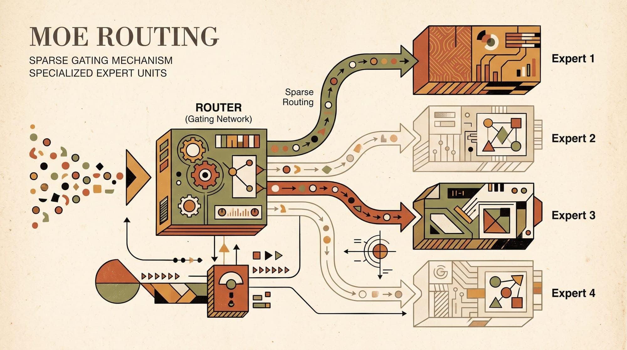
Mixture-of-Experts (MoE) Routing and Load Balancing: Mathematical Foundations of Noisy Top-k Gating, Expert Capacity, Auxiliary Balancing Losses, and Loss-Free Load Balancing

Scaling dense transformer models incurs computational costs that grow proportionally with parameter count. In dense architectures, every token in a sequence activates all feed-forward network (FFN) parameters across every layer. Sparse Mixture-of-Experts (MoE) architectures decouple parameter count from per-token compute by partitioning dense FFN layers into multiple independent sub-networks ("experts") and deploying a learned gating router to direct each token to a sparse subset of experts.

While sparse activation allows models to scale to hundreds of billions or trillions of parameters at the inference and training cost of a much smaller dense model, it introduces a severe optimization instability: routing collapse. Left unconstrained, learned routers naturally degenerate into trivial attractor states where a small fraction of experts receive nearly all tokens, while the remaining experts receive zero gradients and starve.

Addressing routing collapse has driven a ten-year progression in neural architecture design, spanning stochastic noise injection, capacity-constrained communication buffers, auxiliary load-balancing objectives, router stability losses, and recently, auxiliary-loss-free dynamic bias adjustments.

1. Mathematical Formulation of Sparse MoE Gating

In a standard transformer layer, the token representation $x \in \mathbb{R}^{d}$ passes through a Multi-Head Attention (MHA) block followed by a Feed-Forward Network (FFN):

$$\text{FFN}(x) = \sigma(x W_1 + b_1) W_2 + b_2$$

In a sparse MoE layer, the monolithic FFN is replaced by a collection of $N$ parallel expert networks $\{E_1, E_2, \dots, E_N\}$, where each expert $E_i: \mathbb{R}^d \to \mathbb{R}^d$ possesses independent parameter weights $(W_{1}^{(i)}, W_{2}^{(i)})$. A parametric routing module $G: \mathbb{R}^d \to \mathbb{R}^N$ assigns a sparse weighting vector over all $N$ experts.

The layer output is computed as the linearly weighted combination of the selected expert outputs:

$$y = \sum_{i=1}^N G(x)_i E_i(x)$$

Because $G(x)$ is constrained to be sparse (having at most $k \ll N$ non-zero entries), only $k$ expert forward passes are executed per token.

Classical Softmax Routing and Its Failure Mode

The naive implementation of a router computes affine logits followed by a standard softmax distribution:

$$H(x) = x W_g$$

$$G(x) = \text{Softmax}(H(x))$$

where $W_g \in \mathbb{R}^{d \times N}$ is the learnable gating weight matrix. To enforce sparsity, one selects the indices corresponding to the top-$k$ entries in $H(x)$.

Under naive gradient descent, this mechanism exhibits positive feedback loops:

1. If expert $i$ randomly initializes with slightly better representation alignment for a cluster of tokens, it receives higher gating weights $G(x)_i$.
2. Because expert $i$ processes more tokens, its weights receive frequent gradient updates, improving its capability faster than dormant experts.
3. The router observes that expert $i$ minimizes loss more effectively, further increasing gating probabilities toward expert $i$.
4. Dormant experts receive fewer tokens, fewer gradients, and eventually permanently shut down.

2. Noisy Top-k Gating

To break the deterministic positive feedback loop during training, Shazeer et al. (2017) introduced Noisy Top-k Gating. The router injects tunable Gaussian noise into the unnormalized gating logits prior to top-$k$ selection.

Given input $x$, the router evaluates a base affinity logit and a learned per-expert noise scale:

$$H(x)_i = (x W_g)_i + \epsilon \cdot \text{Softplus}((x W_{\text{noise}})_i), \quad \epsilon \sim \mathcal{N}(0, 1)$$

where $W_g \in \mathbb{R}^{d \times N}$ represents the primary gating projection, $W_{\text{noise}} \in \mathbb{R}^{d \times N}$ controls the input-dependent noise magnitude, and $\text{Softplus}(z) = \log(1 + e^z)$ guarantees non-negative standard deviations.

The router then applies a thresholding operation $\text{KeepTopK}(\cdot, k)$ that preserves the $k$ largest values and sets all remaining coordinates to $-\infty$:

$$\text{KeepTopK}(v, k)_i = \begin{cases} v_i & \text{if } v_i \text{ is in the top } k \text{ elements of } v \\ -\infty & \text{otherwise} \end{cases}$$

The final gating distribution is obtained via softmax normalization over the thresholded logits:

$$G(x) = \text{Softmax}(\text{KeepTopK}(H(x), k))$$

Because elements outside the top-$k$ are set to $-\infty$, their softmax probabilities evaluate to exactly zero:

$$G(x)_i = \begin{cases} \frac{\exp(H(x)_i)}{\sum_{j \in \mathcal{K}} \exp(H(x)_j)} & \text{if } i \in \mathcal{K} \\ 0 & \text{if } i \notin \mathcal{K} \end{cases}$$

where $\mathcal{K} = \text{TopKIndices}(H(x), k)$.

Gradient Flow Through Noisy Gating

The non-zero gating weights $G(x)_i$ for $i \in \mathcal{K}$ are smooth and differentiable with respect to $W_g$, $W_{\text{noise}}$, and $x$. The gradient of the task loss $\mathcal{L}$ with respect to the gating logit $H(x)_i$ for an active expert is:

$$\frac{\partial \mathcal{L}}{\partial H(x)_i} = \sum_{j \in \mathcal{K}} \frac{\partial \mathcal{L}}{\partial G(x)_j} \frac{\partial G(x)_j}{\partial H(x)_i} = G(x)_i \left( \frac{\partial \mathcal{L}}{\partial G(x)_i} - \sum_{j \in \mathcal{K}} G(x)_j \frac{\partial \mathcal{L}}{\partial G(x)_j} \right)$$

While the discrete set selection $\mathcal{K}$ introduces non-differentiable boundary transitions, the stochastic noise term $\epsilon \sim \mathcal{N}(0, 1)$ ensures continuous exploration of alternative expert subsets during early optimization.

3. Distributed Hardware Constraints: Expert Capacity and Buffer Overflow

In large-scale distributed training, experts are distributed across separate GPU devices using Expert Parallelism (EP). To maximize hardware utilization on tensor accelerators (NVIDIA GPUs, Google TPUs), computation kernels require static, predetermined tensor dimensions.

If tokens were dynamically routed without limits, an overloaded expert would exceed its allocated memory buffer, causing Out-Of-Memory (OOM) faults or stalling communication collectives.

To guarantee static tensor shapes, Lepikhin et al. (GShard, 2020) and Fedus et al. (Switch Transformers, 2022) formalized the concept of Expert Capacity.

Mathematical Definition of Expert Capacity

Given a batch of $B$ sequences, each with length $S$, the total number of tokens entering an MoE layer is $T = B \times S$. If each token is routed to $k$ experts, the total number of token-expert assignments is $k \times T$.

Under uniform distribution across $N$ experts, each expert expects to receive exactly $\frac{k \cdot T}{N}$ tokens. The Expert Capacity $C$ is defined by scaling this baseline by a capacity factor $f_{\text{capacity}} \ge 1.0$:

$$C = \left\lceil \frac{k \cdot B \cdot S}{N} \cdot f_{\text{capacity}} \right\rceil$$

                          Batch of T Tokens (T = B x S)
                                       │
                                       ▼
                       Learned Gating Router: Top-k(H(x))
                                       │
            ┌──────────────────────────┼──────────────────────────┐
            ▼                          ▼                          ▼
     Expert 1 Buffer            Expert 2 Buffer            Expert N Buffer
     Capacity: C slots          Capacity: C slots          Capacity: C slots
    ┌─────────────────┐        ┌─────────────────┐        ┌─────────────────┐
    │ Token 1         │        │ Token 3         │        │ Token 2         │
    │ Token 4         │        │ Token 7         │        │ Token 5         │
    │ [Pad Slot]      │        │ Token 9         │        │ Token 8         │
    └─────────────────┘        └─────────────────┘        └─────────────────┘
                                       │
                              (If Tokens > C: OVERFLOW)
                                       ▼
                         Dropped Token Bypass (Residual: y = x)

Buffer Overflow and Token Dropping

Each expert allocates a static input buffer of shape $(C, d)$. When tokens are routed to expert $i$:

• If the number of tokens assigned to expert $i$ is less than or equal to $C$, the remaining slots are filled with zero-padding tokens. Padding tokens are ignored during loss computation and gradient backpropagation.
• If the number of assigned tokens exceeds $C$, the excess tokens are dropped. A dropped token bypasses the expert computation entirely and is passed directly to the next layer via the identity residual connection ($y = x$).

The capacity factor $f_{\text{capacity}}$ embodies a fundamental engineering trade-off:

• Low Capacity Factor ($f_{\text{capacity}} = 1.0$): Zero memory waste on padding, but high token drop rates whenever routing distribution drifts from uniform balance. Dropped tokens degrade language modeling perplexity.
• High Capacity Factor ($f_{\text{capacity}} \ge 1.5\text{--}2.0$): Eliminates token dropping at the expense of allocating substantial GPU memory to idle zero-padding, reducing effective batch throughput.

4. Auxiliary Load Balancing Losses

Because token dropping hurts model convergence, MoE architectures introduce auxiliary regularization terms to force the gating network toward uniform token distribution across all available experts.

The Switch Transformer Auxiliary Loss

In the Switch Transformer, Fedus et al. formulated a clean, differentiable auxiliary loss. For a given batch containing $T$ tokens, two metrics are computed for each expert $i \in \{1, \dots, N\}$:

1. Fraction of Routed Tokens ($f_i$): The proportion of total routing decisions assigned to expert $i$:

$$f_i = \frac{1}{k \cdot T} \sum_{t=1}^T \sum_{j=1}^k \mathbb{I}(\text{Expert } i \text{ is the } j\text{-th choice for token } t)$$

where $\mathbb{I}(\cdot)$ is the indicator function.

1. Average Routing Probability ($P_i$): The mean softmax gating probability allocated to expert $i$ across all tokens in the batch:

$$P_i = \frac{1}{T} \sum_{t=1}^T G(x_t)_i$$

The auxiliary load balancing loss $\mathcal{L}_{\text{aux}}$ is defined as the scaled inner product of the vectors $f$ and $P$:

$$\mathcal{L}_{\text{aux}} = \alpha \cdot N \sum_{i=1}^N f_i \cdot P_i$$

where $\alpha$ is a hyperparameter (typically $\alpha \in [10^{-3}, 10^{-2}]$).

Proof of Uniform Minimum

The product $f_i P_i$ couples the non-differentiable assignment count $f_i$ with the differentiable probability mass $P_i$.

By the Cauchy-Schwarz inequality, for any non-negative probability vectors $f, P \in \Delta^{N-1}$ (where $\sum f_i = 1$ and $\sum P_i = 1$):

$$\sum_{i=1}^N f_i P_i \ge \frac{1}{N} \left( \sum_{i=1}^N \sqrt{f_i P_i} \right)^2$$

When $f = P$, this simplifies to:

$$\sum_{i=1}^N f_i^2 \ge \frac{1}{N} \left( \sum_{i=1}^N f_i \right)^2 = \frac{1}{N}$$

The global minimum of $\sum_{i=1}^N f_i P_i$ is achieved if and only if:

$$f_1 = f_2 = \dots = f_N = \frac{1}{N} \quad \text{and} \quad P_1 = P_2 = \dots = P_N = \frac{1}{N}$$

At this balanced point:

$$\mathcal{L}_{\text{aux}} = \alpha \cdot N \sum_{i=1}^N \left( \frac{1}{N} \cdot \frac{1}{N} \right) = \alpha \cdot N \left( N \cdot \frac{1}{N^2} \right) = \alpha$$

If any expert attracts disproportionate traffic (e.g., $f_k \gg 1/N$), both $f_k$ and $P_k$ increase simultaneously, driving up $\mathcal{L}_{\text{aux}}$ quadratically and penalizing the router weights $W_g$.

Imbalance State: Expert 1 gets 70% of tokens, Experts 2-4 get 10% each
f = [0.70, 0.10, 0.10, 0.10], P = [0.70, 0.10, 0.10, 0.10]
L_aux = α * 4 * (0.49 + 0.01 + 0.01 + 0.01) = α * 4 * 0.52 = 2.08 α

Balanced State: Experts 1-4 get 25% of tokens each
f = [0.25, 0.25, 0.25, 0.25], P = [0.25, 0.25, 0.25, 0.25]
L_aux = α * 4 * (0.0625 * 4) = α * 4 * 0.25 = 1.00 α

5. Router Numerical Stability: The Z-Loss

During large-scale pre-training of deep MoE models (such as ST-MoE, Zoph et al., 2022), routers frequently experience logit drift. Because the softmax operation is translation invariant:

$$\text{Softmax}(z) = \text{Softmax}(z - c \cdot \mathbf{1})$$

the routing logits $H(x)_i = (x W_g)_i$ can grow to extreme positive values ($> 10^3$) without changing the resulting softmax probabilities. In 16-bit floating point formats (FP16 or BF16), large logit magnitudes cause catastrophic exponent overflow, yielding NaN activations that corrupt training checkpoints.

To maintain logit magnitudes within stable numerical ranges, ST-MoE introduced the Router Z-Loss:

$$\mathcal{L}_{z} = c_z \cdot \frac{1}{T} \sum_{t=1}^T \left( \log \sum_{j=1}^N \exp(H(x_t)_j) \right)^2$$

where $c_z$ is a small weighting coefficient (typically $c_z \in [10^{-4}, 10^{-3}]$).

The Z-loss directly penalizes the logarithm of the softmax partition function (the log-sum-exp of logits). By driving large logit values toward zero, the Z-loss eliminates floating-point round-off errors and prevents gradient divergence across billions of tokens.

6. Token-Choice vs. Expert-Choice Routing

All top-$k$ architectures discussed above operate under Token-Choice Routing: individual tokens evaluate all experts and select the top-$k$ candidates.

In 2022, Zhou et al. (Google Brain) inverted this formulation by introducing Expert-Choice Routing.

Token-Choice Routing:
  Each token selects Top-k experts.
  Result: Variable expert load (some experts overflow, others starve).
  Remedy: Capacity factor padding and auxiliary balancing losses.

Expert-Choice Routing:
  Each expert selects Top-C tokens.
  Result: Perfect expert load balance by construction (exactly C tokens per expert).
  Consequence: Variable token allocation (some tokens get multiple experts, some get none).

Expert-Choice Mathematical Formulation

Let $X \in \mathbb{R}^{T \times d}$ represent the concatenated matrix of all $T$ tokens in a batch. The router computes a token-to-expert affinity score matrix $S \in \mathbb{R}^{T \times N}$:

$$S = \text{Softmax}_{\text{tokens}}(X W_g)$$

where the softmax is computed column-wise across the token dimension $T$, rather than row-wise across experts:

$$S_{t, e} = \frac{\exp((x_t W_g)_e)}{\sum_{\tau=1}^T \exp((x_\tau W_g)_e)}$$

Each expert $e \in \{1, \dots, N\}$ selects the top-$C$ tokens with the highest affinity scores in column $e$:

$$\mathcal{T}_e = \text{TopKIndices}(S_{:, e}, C)$$

Because every expert selects exactly $C$ tokens, every expert buffer is filled to 100% capacity with zero padding and zero dropped tokens.

Trade-Offs of Expert-Choice Routing

While Expert-Choice routing achieves optimal FLOP efficiency and hardware utilization, it introduces two fundamental architectural constraints:

1. Uneven Token Representation: Important tokens (e.g., subject nouns or syntax roots) may be selected by 5 or 6 experts simultaneously, while simple tokens (e.g., punctuation or articles) may be selected by 0 experts, relying solely on residual connections.
2. Causal Autoregressive Decoding Incompatibility: During autoregressive inference (step-by-step generation), future tokens do not exist. An expert cannot compute the top-$C$ tokens across a batch until all tokens have arrived. Consequently, Expert-Choice routing is well-suited for encoder and prefill models, but cannot be applied directly to standard causal next-token generation loops.

7. Fine-Grained Segmentation and Shared Experts

To improve expert specialization without inflating routing complexity, modern architectures have transitioned from coarse experts to fine-grained expert segmentation combined with dedicated shared experts. This paradigm was formalized in DeepSeekMoE (Dai et al., 2024).

Fine-Grained Expert Partitioning

Instead of deploying $N$ large experts with hidden dimension $d_{\text{ffn}}$ and routing top-$k$, DeepSeekMoE splits each expert into $m$ smaller sub-experts with intermediate dimension $d_{\text{ffn}} / m$. The total number of experts becomes $m N$, and the router selects top-$m k$ sub-experts:

Standard MoE (e.g., Mixtral 8x7B):
  Total Experts: N = 8
  Active Experts: k = 2
  Combinations: C(8, 2) = 28 routing paths

Fine-Grained MoE (DeepSeekMoE, m = 4):
  Total Experts: 4 * 8 = 32
  Active Experts: 4 * 2 = 8
  Combinations: C(32, 8) = 10,518,300 routing paths

With identical parameter count and computational FLOPs per forward pass, fine-grained partitioning expands the combinatorial capacity of the model by several orders of magnitude, allowing sub-experts to learn highly focused, disentangled features.

Dedicated Shared Experts

In standard MoE models, redundant common knowledge (e.g., English grammar rules, punctuation syntax, common code structure) must be duplicated across all independent experts to prevent performance degradation when routed.

DeepSeekMoE isolates this invariant knowledge by reserving $K_{\text{shared}}$ experts that are always activated for every token, irrespective of router scores. The remaining $K_{\text{routed}}$ slots are dynamically allocated via top-$k$ gating:

$$y = \sum_{j=1}^{K_{\text{shared}}} E_{j}^{\text{shared}}(x) + \sum_{i \in \text{TopK}} G(x)_i E_{i}^{\text{routed}}(x)$$

By delegating general-purpose representations to fixed shared pathways, dynamic routed experts specialize purely in niche domain capabilities (e.g., specific programming languages, mathematical theorems, or multilingual translations).

8. Auxiliary-Loss-Free Load Balancing

While auxiliary load balancing losses ($\mathcal{L}_{\text{aux}} = \alpha N \sum f_i P_i$) prevent expert starvation, they introduce a fundamental structural conflict:

$$\nabla_{\theta} \mathcal{L}_{\text{total}} = \nabla_{\theta} \mathcal{L}_{\text{LM}} + \alpha \nabla_{\theta} \mathcal{L}_{\text{aux}}$$

The gradient of the language modeling loss $\nabla \mathcal{L}_{\text{LM}}$ attempts to route tokens to the expert most capable of predicting the next token. Simultaneously, the gradient of the auxiliary loss $\nabla \mathcal{L}_{\text{aux}}$ forces the router to route tokens away from capable experts to equalize traffic.

When $\alpha$ is too small ($\alpha \le 10^{-4}$), load balancing fails, causing expert collapse and token dropping. When $\alpha$ is too large ($\alpha \ge 10^{-2}$), gradient interference severely degrades validation perplexity.

To resolve this conflict, Wang et al. (DeepSeek, 2024) developed Auxiliary-Loss-Free Load Balancing, deployed in DeepSeek-V3.

                    ┌──────────────────────────────────────┐
                    │ Input Token Representation x ∈ R^d   │
                    └──────────────────┬───────────────────┘
                                       │
                         ┌─────────────┴─────────────┐
                         │ Affine Projection: x * Wg │
                         └─────────────┬─────────────┘
                                       │
                 ┌─────────────────────┴─────────────────────┐
                 │                                           │
                 ▼                                           ▼
   Logit + Dynamic Bias b_i                      Raw Affinity Logits (Unbiased)
   (Used ONLY for Expert Selection)              (Used ONLY for Softmax Gating Weights)
                 │                                           │
                 ▼                                           │
   Select Top-k Indices K                                    │
   K = TopK(x * Wg + b, k)                                   │
                 │                                           │
                 └─────────────────────┬─────────────────────┘
                                       │
                                       ▼
                     Compute Normalized Gating Probabilities
                     G(x)_i = Softmax_{j ∈ K}( (x * Wg)_j )
                                       │
                                       ▼
                     Zero Auxiliary Loss Gradients on Router

Dynamic Bias Adjustment Mechanism

Instead of adding a penalty term to the backward loss graph, the router introduces a learnable per-expert bias vector $b \in \mathbb{R}^N$ that is updated dynamically based on real-time hardware queue statistics.

1. Top-k Selection with Bias: When routing token $x$, the top-$k$ expert indices are selected using the bias-augmented affinity scores:

$$\mathcal{K} = \text{TopKIndices}(x W_g + b, k)$$

1. Gating Weight Calculation without Bias: Once the expert indices $\mathcal{K}$ are selected, the actual gating weights $G(x)_i$ used to multiply expert outputs are computed using the original, unbiased logits:

$$G(x)_i = \begin{cases} \frac{\exp((x W_g)_i)}{\sum_{j \in \mathcal{K}} \exp((x W_g)_j)} & \text{if } i \in \mathcal{K} \\ 0 & \text{if } i \notin \mathcal{K} \end{cases}$$

Because $b$ is excluded from the softmax denominator, the scale of $G(x)_i$ reflects pure model-driven confidence rather than artificial routing corrections.

1. Runtime Bias Update Rule: At the end of each training step $t$, the bias term $b_i$ for each expert is adjusted directly based on its observed token load $C_i^{(t)}$ relative to the target average load $\bar{C} = \frac{k T}{N}$:

$$b_i^{(t+1)} = b_i^{(t)} + \gamma \cdot \text{sgn}\left( \bar{C} - C_i^{(t)} \right)$$

where $\gamma > 0$ is a fixed step size (typically $\gamma \in [10^{-4}, 10^{-3}]$), and $\text{sgn}(\cdot)$ denotes the signum function:

• If expert $i$ is underloaded ($C_i^{(t)} < \bar{C}$), $b_i$ increases, raising the probability that expert $i$ enters the top-$k$ in subsequent steps.
• If expert $i$ is overloaded ($C_i^{(t)} > \bar{C}$), $b_i$ decreases, throttling incoming token traffic.

Why Loss-Free Balancing Outperforms Auxiliary Losses

1. Zero Gradient Interference: Because $b$ is updated as an external control variable rather than via autograd backpropagation, $\nabla_{W_g} \mathcal{L}_{\text{aux}} = 0$. The routing projection $W_g$ updates solely to minimize the primary language modeling cross-entropy $\mathcal{L}_{\text{LM}}$.
2. Deterministic Load Convergence: Unlike stochastic gradient descent which oscillates around auxiliary loss landscapes, the signum control loop acts as an integral feedback controller, maintaining expert utilization within $\pm 2\%$ of perfect parity throughout training.
3. Elimination of Dropped Tokens: Perfect load parity allows distributed clusters to operate at $f_{\text{capacity}} = 1.05$ with zero token drops, reducing memory allocation overhead while preserving maximum downstream reasoning performance.

9. Architectural Comparison of MoE Routing Paradigms

| Routing Mechanism | Gating Formulation | Load Balancing Method | Dropped Tokens | Gradient Interference | Primary Production Implementations | | :--- | :--- | :--- | :--- | :--- | :--- | | Noisy Top-k Gating | $\text{TopK}(x W_g + \epsilon \cdot \text{Softplus}(x W_{\text{noise}}), k)$ | Stochastic Gaussian noise exploration | Yes (High under load imbalance) | Minimal | Shazeer et al. (2017) | | Switch Routing | $\text{Top1}(x W_g)$ | Auxiliary Loss ($\alpha N \sum f_i P_i$) | Yes (If $T_i > C$) | Moderate | Switch Transformer | | ST-MoE Gating | $\text{Top2}(x W_g)$ | Auxiliary Loss + Router Z-Loss | Yes (Low with capacity slack) | Moderate | ST-MoE, PaLM-2 MoE | | Expert-Choice | $\text{TopC}_{\text{tokens}}(X W_g)$ | Column-wise token selection | No (0% by construction) | None | Zhou et al. (2022) | | Fine-Grained + Shared | $\sum E_{\text{shared}} + \text{TopK}(x W_g, k)$ | Auxiliary Loss + Shared Invariant Routing | Yes (Bounded) | Low-to-Moderate | DeepSeekMoE, Qwen-MoE | | Auxiliary-Loss-Free | $\text{TopK}(x W_g + b, k)$ with unperturbed $G(x)$ | Dynamic signum bias control loop ($b \leftarrow b + \gamma \Delta C$) | No (Zero drop at $f_{\text{cap}} \approx 1.0$) | None (Zero) | DeepSeek-V3, DeepSeek-R1 |

10. Summary and Implementation Takeaways

The evolution of Mixture-of-Experts routing reflects a continuous push toward eliminating artificial constraints on the language modeling objective:

1. Routing Collapse is an Inherent Dynamic of Softmax Selection: Naive gradient descent on sparse gating layers inevitably produces winner-take-all routing.
2. Auxiliary Losses are a Compromise: While inner-product auxiliary penalties ($f_i P_i$) force equal distribution, their gradient backpropagation actively conflicts with task performance, forcing a compromise between hardware efficiency and token perplexity.
3. Z-Loss Resolves Precision Instability: Adding a squared log-partition regularizer prevents logit magnitude explosion, protecting FP16/BF16 training stability across deep layers.
4. Shared Experts Prevent Redundant Parameter Allocation: Dedicated invariant experts absorb general language representations, allowing routed experts to focus entirely on orthogonal specialized domains.
5. Dynamic Biases Decouple Load Control from Representation Learning: Shifting load balancing from loss-function gradient backpropagation to runtime feedback control (as in DeepSeek-V3) achieves hardware load balancing without degrading language modeling quality.

Sources

• Shazeer, N., Mirhoseini, A., Maziarz, K., Davis, A., Le, Q., Hinton, G., & Dean, J. (2017). Outrageously Large Neural Networks: The Sparsely-Gated Mixture-of-Experts Layer. arXiv:1701.06538.
• Lepikhin, D., Lee, H., Xu, Y., Chen, D., Firat, O., Yadav, Y., ... & Chen, Z. (2020). GShard: Scaling Giant Models with Conditional Computation and Automatic Sharding. ICLR 2021.
• Fedus, W., Zoph, B., & Shazeer, N. (2022). Switch Transformers: Scaling to Trillion Parameter Models with Simple and Efficient Sparsity. Journal of Machine Learning Research (JMLR).
• Zoph, B., Bello, I., Kumar, S., Du, N., Huang, D., Dean, J., ... & Fedus, W. (2022). ST-MoE: Designing Stable and Transferable Sparse Expert Models. arXiv:2202.08906.
• Zhou, Y., Lei, T., Liu, H., Du, N., Huang, D., Zhao, V. Y., ... & Le, Q. V. (2022). Mixture-of-Experts with Expert Choice Routing. NeurIPS 2022.
• Dai, D., Deng, C., Zhao, C., Xu, R. X., Gao, H., Chen, D. L., ... & Liang, W. (2024). DeepSeekMoE: Towards Ultimate Expert Specialization in Mixture-of-Experts Language Models. arXiv:2401.06066.
• Wang, P., et al. (2024). Auxiliary-Loss-Free Load Balancing Strategy for Mixture-of-Experts. arXiv:2408.15664.