Low-Rank Adaptation (LoRA) and QLoRA: Mathematical Foundations, Intrinsic Rank Dynamics, NF4 Quantization, and Parameter-Efficient Fine-Tuning

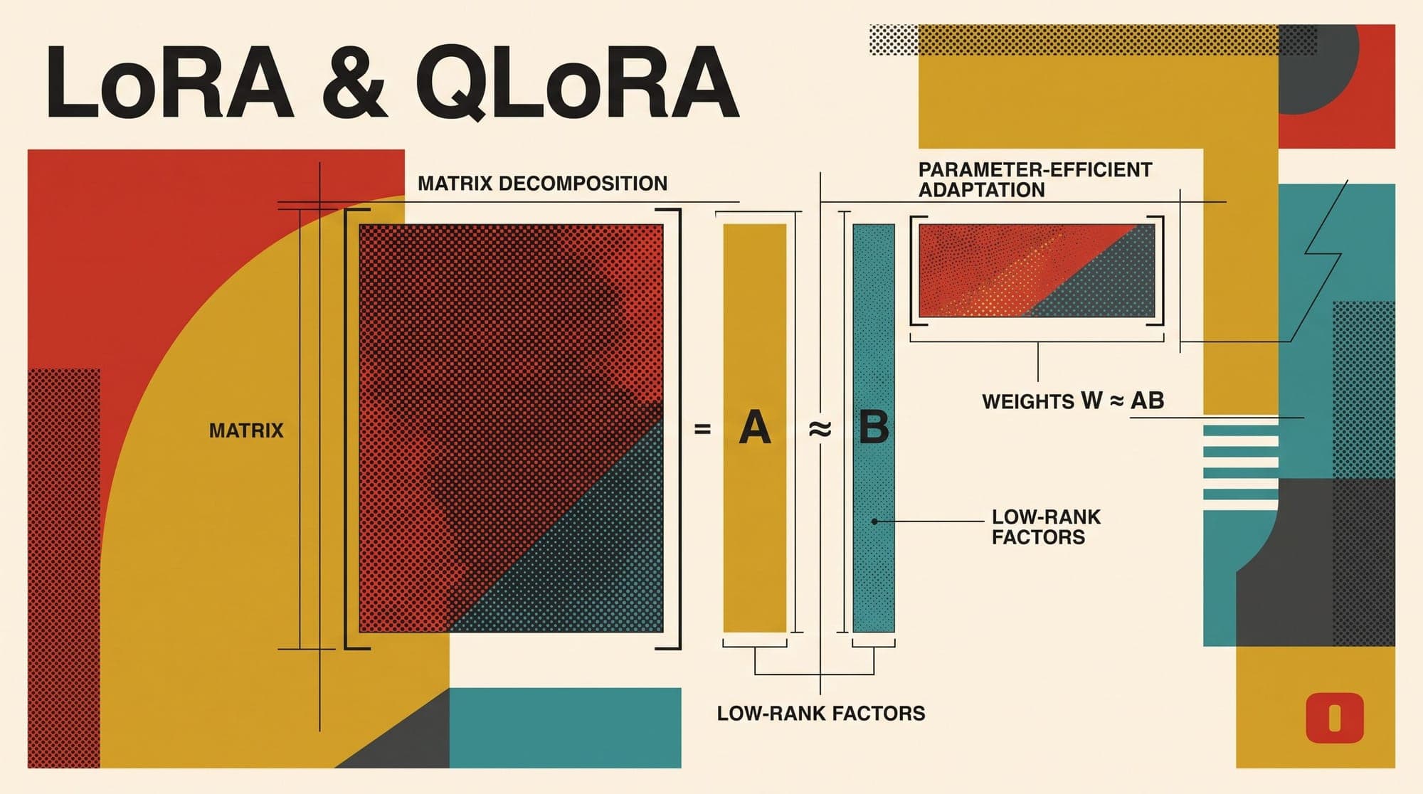
Full fine-tuning of large language models requires updating every parameter matrix across all transformer blocks. In production architectures spanning tens to hundreds of billions of parameters, the computational and memory footprint of updating billions of weights with first-order and second-order optimizer states becomes prohibitive.

Low-Rank Adaptation (LoRA) and its quantized counterpart QLoRA provide mathematically grounded parameter-efficient fine-tuning (PEFT) frameworks. By decomposing dense weight update matrices into low-rank factorizations and leveraging information-theoretically optimal non-linear data types, these methods compress the trainable parameter footprint by multiple orders of magnitude while preserving full fine-tuning performance.

The Memory Bottleneck of Full Fine-Tuning

During full parameter fine-tuning with 16-bit precision (FP16 or BF16) using standard AdamW optimization, the total VRAM required per parameter extends far beyond the static model weights:

• Model weights: 2 bytes per parameter (16-bit float).
• Gradients: 2 bytes per parameter.
• AdamW optimizer states: 4 bytes for the master copy of weights in FP32, 4 bytes for the first momentum estimate ($m$), and 4 bytes for the second raw variance estimate ($v$).
• Total static memory: 16 bytes per parameter.

For a 70-billion parameter base model, storing the model weights, gradients, and optimizer states requires 1.12 TB of high-bandwidth memory (HBM) before accounting for sequence activations, KV caches, or intermediate tensor allocations. Distributed training across a cluster of 8x 80 GB GPUs using Fully Sharded Data Parallel (FSDP) or DeepSpeed ZeRO-3 is necessary solely to hold the state.

LoRA addresses this memory wall by freezing the pre-trained weight matrices $W_0$ and introducing low-rank trainable decomposition matrices. Because $W_0$ remains static, no gradients or optimizer states are allocated for the base model, eliminating over 75 percent of the static memory requirement.

Intrinsic Dimensionality and Low-Rank Parameter Dynamics

The theoretical justification for low-rank adaptation stems from empirical and theoretical findings regarding the intrinsic dimensionality of overparameterized neural networks. Aghajanyan et al. (2020) demonstrated that pre-trained language models reside on a low-dimensional optimization manifold: the objective function can be effectively minimized within a randomly projected subspace of dimension $d_{int} \ll D_{total}$.

Building on this insight, Hu et al. (2021) hypothesized that the task-specific weight updates $\Delta W$ during adaptation also possess a low intrinsic rank. For a pre-trained weight matrix $W_0 \in \mathbb{R}^{d_{out} \times d_{in}}$, full fine-tuning computes an unconstrained update matrix $\Delta W \in \mathbb{R}^{d_{out} \times d_{in}}$ where the rank of $\Delta W$ is bounded only by $\min(d_{in}, d_{out})$.

LoRA constrains the rank of $\Delta W$ explicitly by parameterizing it as the product of two low-rank matrices $B$ and $A$:

$$\Delta W = B A$$

Where $B \in \mathbb{R}^{d_{out} \times r}$, $A \in \mathbb{R}^{r \times d_{in}}$, and the adaptation rank $r$ satisfies $r \ll \min(d_{in}, d_{out})$.

For a linear transformation with input vector $x \in \mathbb{R}^{d_{in}}$, the modified forward pass is computed as:

$$h = W_0 x + \Delta W x = W_0 x + \frac{\alpha}{r} B A x$$

Here, $\alpha$ is a constant scaling hyperparameter.

                  +--------------------------+
                  |      Input Vector x      |
                  +--------------------------+
                       /                \
                      /                  \
                     v                    v
          +--------------------+   +---------------+
          | Frozen Base Weight |   | Trainable A   |  (r x d_in)
          |        W_0         |   +---------------+
          |   (d_out x d_in)   |          |
          +--------------------+          v
                     |             +---------------+
                     |             | Trainable B   |  (d_out x r)
                     |             +---------------+
                     |                    |
                     |                    v
                     |             +---------------+
                     |             | Scale (alpha/r)|
                     |             +---------------+
                     \                    /
                      \                  /
                       v                v
                  +--------------------------+
                  |  Summation h = W0*x + BAx|
                  +--------------------------+

Initialization and the Scaling Factor

The initialization scheme for $A$ and $B$ is critical to ensure training stability and preserve pre-trained capabilities at the start of adaptation:

1. Matrix $A$ is initialized using a random Gaussian distribution $\mathcal{N}(0, \sigma^2)$ (or Kaiming uniform initialization).
2. Matrix $B$ is initialized entirely to zero ($B = 0$).

At initialization step $t=0$:

$$\Delta W = B A = 0 \cdot A = 0$$

As a result, $h = W_0 x$, meaning the model output exactly matches the pre-trained model at the start of training, avoiding destructive gradient shocks on the first forward pass.

The hyperparameter $\alpha$ acts as a constant scaling factor. When tuning the adaptation rank $r$, scaling the update by $\frac{\alpha}{r}$ stabilizes the expected magnitude of the adapter's contribution. When $r$ is increased or decreased, the effective learning rate across the adapter parameters does not require extensive re-tuning, as the scaling factor automatically adjusts the magnitude of $\Delta W x$.

Gradient Dynamics and Backpropagation Mechanics

During backpropagation, the gradients of the task loss $\mathcal{L}$ with respect to the adapter matrices $A$ and $B$ are computed directly via the chain rule.

Given output activation $y = h = W_0 x + \frac{\alpha}{r} B A x$ and upstream gradient $\frac{\partial \mathcal{L}}{\partial y} \in \mathbb{R}^{1 \times d_{out}}$:

$$\frac{\partial \mathcal{L}}{\partial B} = \frac{\alpha}{r} \left(\frac{\partial \mathcal{L}}{\partial y}\right)^T (A x)^T \in \mathbb{R}^{d_{out} \times r}$$

$$\frac{\partial \mathcal{L}}{\partial A} = \frac{\alpha}{r} B^T \left(\frac{\partial \mathcal{L}}{\partial y}\right)^T x^T \in \mathbb{R}^{r \times d_{in}}$$

To pass the gradient downstream to earlier transformer layers, the gradient with respect to the input activation $x$ is computed:

$$\frac{\partial \mathcal{L}}{\partial x} = \left(W_0 + \frac{\alpha}{r} B A\right)^T \left(\frac{\partial \mathcal{L}}{\partial y}\right)^T \in \mathbb{R}^{d_{in} \times 1}$$

Because $W_0$ is frozen:

• No gradient $\frac{\partial \mathcal{L}}{\partial W_0}$ is accumulated in memory.
• No optimizer states (momentum or variance) are stored for $W_0$.
• The base weight $W_0$ is accessed only during the forward GEMM and the backward activation gradient GEMM.

Target Module Allocation and Subspace Overlap

The original LoRA implementation focused primarily on the multi-head self-attention projection matrices: the query projection $W_q$, key projection $W_k$, value projection $W_v$, and output projection $W_o$.

Subsequent empirical studies across standard foundation models revealed key structural insights:

1. Targeting All Linear Projections: Applying LoRA with a small rank (such as $r=8$ or $r=16$) across all linear projection layers—including attention projections ($W_q, W_k, W_v, W_o$) and MLP feed-forward projections ($W_{gate}, W_{up}, W_{down}$)—consistently outperforms applying a higher rank ($r=64$) strictly to $W_q$ and $W_v$.
2. Singular Value Distribution: SVD analysis on learned $\Delta W$ matrices indicates that a small number of singular vectors capture the vast majority of the variance. The top singular values dominate the adaptation dynamic, while remaining dimensions exhibit near-zero singular values, validating the low-rank hypothesis.
3. Grassmann Distance and Subspace Similarity: When training adapters with different ranks $r_1 < r_2$, the subspace spanned by the columns of $A$ and $B$ in $r_1$ shares significant directional overlap with the top $r_1$ singular vectors of the adapter trained with $r_2$.

QLoRA: 4-Bit NormalFloat and Memory Optimization

While standard LoRA eliminates optimizer states for the base model, the static base model weights $W_0$ must still reside in VRAM. For a 65B or 70B model in 16-bit precision, the base weights alone occupy 130 to 140 GB of VRAM.

Dettmers et al. (2023) introduced QLoRA, which integrates 4-bit base model quantization with 16-bit low-rank adapters. QLoRA introduces three core algorithmic mechanisms:

1. 4-bit NormalFloat (NF4) Quantization

Standard integer quantization (such as uniform INT4) is suboptimal for neural network weights, which follow a Gaussian distribution centered at zero: $W_{ij} \sim \mathcal{N}(0, \sigma^2)$.

NF4 is an information-theoretically optimal quantile quantization data type constructed such that each 4-bit quantization bin contains an equal number of expected parameters under a zero-mean standard normal distribution.

The $2^k$ quantization bins $q_i$ (for $k=4$, $2^4 = 16$ levels) are derived from the empirical quantile function $Q_X(\cdot)$ of the standard normal distribution $\mathcal{N}(0, 1)$:

$$q_i = \frac{1}{2}\left(Q_X\left(\frac{i}{2^k}\right) + Q_X\left(\frac{i+1}{2^k}\right)\right)$$

The resulting discrete points are normalized to the symmetric interval $[-1, 1]$. To quantize a weight tensor block $W \in \mathbb{R}^{B_{block}}$:

1. Compute the absolute maximum scale: $c = \max(|W|)$.
2. Normalize the block weights: $\tilde{W} = \frac{W}{c} \in [-1, 1]$.
3. Map each normalized weight $\tilde{w}_{ij}$ to the nearest discrete quantile $q_k$.

During the forward pass, the 4-bit NF4 weights are dequantized on the fly into 16-bit Brain Floating Point (BF16) or FP16 before performing the matrix multiplication with the input activation $x$.

2. Double Quantization (DQ)

Block quantization requires storing a 32-bit floating-point scale factor $c_1^{FP32}$ for every block of parameters (e.g., block size $B_1 = 64$). This creates an auxiliary memory overhead:

$$\text{Overhead} = \frac{32 \text{ bits}}{64 \text{ parameters}} = 0.5 \text{ bits per parameter}$$

Double Quantization treats the first-stage quantization constants $c_1$ as inputs to a second quantization stage with an 8-bit FP8 format and block size $B_2 = 256$:

1. Compute second-stage scale factor $c_2^{FP32}$ over 256 first-stage constants.
2. Quantize $c_1$ to 8-bit integers or FP8: $c_1^{8bit} = \text{round}\left(\frac{c_1}{c_2} \cdot 127\right)$.

This reduces the quantization metadata footprint:

$$\text{Overhead}_{DQ} = \frac{8 \text{ bits}}{64} + \frac{32 \text{ bits}}{64 \times 256} = 0.125 + 0.00195 \approx 0.127 \text{ bits per parameter}$$

Double Quantization saves roughly 0.373 bits per parameter, freeing approximately 3 GB of VRAM on a 65B parameter model.

3. Paged Optimizers

During long-sequence fine-tuning, activation memory requirements fluctuate dynamically, causing sporadic memory spikes that trigger CUDA out-of-memory errors.

QLoRA employs CUDA Unified Memory to automatically allocate page tables for adapter optimizer states. When an allocation spike occurs, non-active optimizer state pages are paged out from GPU HBM to host CPU RAM and paged back asynchronously when required for the gradient update step.

Advanced Variants: DoRA and LoRA+

Following LoRA and QLoRA, architectural refinements have resolved specific training dynamics:

• Weight-Decomposed Low-Rank Adaptation (DoRA): Liu et al. (2024) decomposes the weight matrix into magnitude $m \in \mathbb{R}^{1 \times d_{in}}$ and directional matrix $V \in \mathbb{R}^{d_{out} \times d_{in}}$:

$$W = m \frac{V + \Delta W}{\|V + \Delta W\|_F}$$ This decoupling replicates full fine-tuning dynamics more closely by allowing independent directional updates without unintended scaling distortions.

• LoRA+ (Learning Rate Ratio Scaling): Hayou et al. (2024) demonstrated that when $d_{in}, d_{out} \gg r$, optimizing matrices $A$ and $B$ with the same learning rate leads to sub-optimal feature learning, as $B$ updates more slowly than $A$. Setting $\eta_B = \lambda \eta_A$ (where $\lambda = 2^{2}$ to $2^{4}$) improves convergence speed and downstream task accuracy.

Production Serving and Multi-Tenant Routing

A major operational benefit of LoRA is the ability to eliminate inference latency overhead at deployment.

1. Static Weight Merging

For single-task deployment, the adapter weights can be permanently fused into the base model weights prior to serialization:

$$W_{merged} = W_0 + \frac{\alpha}{r} B A$$

Because matrix addition is associative, the fused model has the exact tensor dimensions, memory footprint, and computational latency of the original unadapted foundation model. Zero additional floating-point operations or memory reads are required during inference.

2. Multi-Tenant Dynamic Multiplexing

In enterprise deployments serving dozens or hundreds of specialized downstream tasks, hosting separate full-model instances is economically impractical. Systems such as S-LoRA (Sheng et al., 2023) and Punica maintain a single frozen base model in GPU VRAM and dynamically route incoming requests to lightweight adapter weights loaded into a unified memory pool.

Batched inference engines utilize Segmented GEMM (SGEMM) kernels to compute base projections concurrently while applying distinct $B_i A_i$ adapter paths to individual sequences within the same batch.

Summary

Low-Rank Adaptation establishes that deep foundation models do not require full parameter perturbation to acquire specialized domain skills. By constraining updates to low-rank subspaces and combining non-linear quantile quantization with memory-managed optimizer states, LoRA and QLoRA reduce hardware requirements by orders of magnitude while preserving foundational performance.

Sources

• Hu, E. J., Shen, Y., Wallis, P., Allen-Zhu, Z., Li, Y., Wang, S., Wang, L., & Chen, W. (2021). LoRA: Low-Rank Adaptation of Large Language Models. arXiv:2106.09685. https://arxiv.org/abs/2106.09685
• Dettmers, T., Pagnoni, A., Holtzman, A., & Zettlemoyer, L. (2023). QLoRA: Efficient Finetuning of Quantized LLMs. arXiv:2305.14314. https://arxiv.org/abs/2305.14314
• Aghajanyan, A., Gupta, S., & Zettlemoyer, L. (2020). Intrinsic Dimensionality Explains the Effectiveness of Language Model Fine-Tuning. arXiv:2012.13255. https://arxiv.org/abs/2012.13255
• Liu, S., Wang, C. Y., Yin, H., Molchanov, P., & Kautz, J. (2024). DoRA: Weight-Decomposed Low-Rank Adaptation. arXiv:2402.09353. https://arxiv.org/abs/2402.09353
• Hayou, S., Ghosh, N., & Yu, B. (2024). LoRA+: Efficient Low Rank Adaptation of Large Models. arXiv:2402.12354. https://arxiv.org/abs/2402.12354
• Sheng, J., et al. (2023). S-LoRA: Serving Thousands of Concurrent LoRA Adapters. arXiv:2311.03285. https://arxiv.org/abs/2311.03285