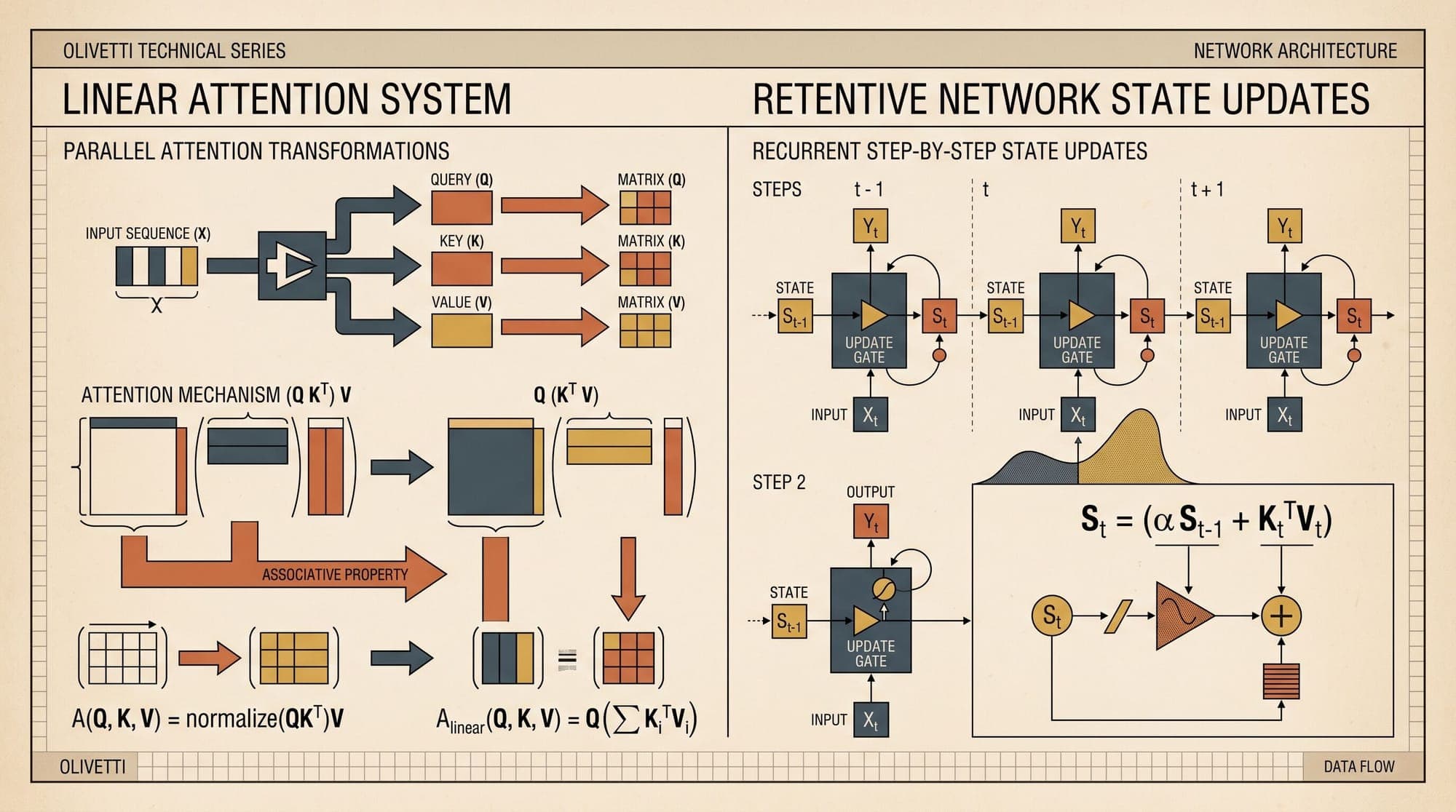
Linear Attention and Retentive Networks: How Recurrent Duals and Chunkwise Tiling Eliminate the Quadratic Bottleneck

Autoregressive large language models built on standard multi-head self-attention face two fundamental scaling ceilings: quadratic compute and memory complexity during pre-training, and linearly expanding key-value (KV) cache memory footprints during autoregressive generation. While optimizations such as FlashAttention reduce memory access overheads and Grouped-Query Attention (GQA) compresses KV projection channels, the core mechanics of softmax attention remain fundamentally bound to sequence length.

Linear attention mechanisms and modern recurrent architectures, exemplified by Retentive Networks (RetNet) and Gated Linear Attention (GLA), resolve this bottleneck by exploiting the mathematical duality between attention and recurrence. By replacing non-linear softmax normalization with kernel feature maps, exponential decay matrices, and data-dependent gating, these architectures achieve the "impossible triangle" of sequence modeling: parallel training at GPU scale, constant $O(1)$ memory and latency during inference, and competitive language modeling perplexity.

The Quadratic Dilemma of Softmax Attention

Standard scaled dot-product attention computes interactions between queries $Q \in \mathbb{R}^{N \times d}$, keys $K \in \mathbb{R}^{N \times d}$, and values $V \in \mathbb{R}^{N \times d}$ across sequence length $N$:

$$\text{Attention}(Q, K, V) = \text{softmax}\left(\frac{Q K^T}{\sqrt{d}}\right) V$$

The intermediate matrix $A = Q K^T \in \mathbb{R}^{N \times N}$ requires materializing or evaluating $N^2$ pairwise interactions. During training, backpropagating through this $N \times N$ matrix requires $O(N^2)$ memory (or $O(N^2)$ recomputation in IO-aware kernels).

Standard Softmax Attention (Autoregressive Generation):
Token 1 ──► [K1, V1] ───┐
Token 2 ──► [K2, V2] ───┼──► KV Cache Grows O(N) ──► Softmax(q_t @ K^T) @ V
Token 3 ──► [K3, V3] ───┤                            (O(N) latency & memory per step)
Token t ──► [Kt, Vt] ───┘

Linear Attention / Retention (Autoregressive Generation):
Token t ──► k_t^T @ v_t ──► [ State Matrix S_t ] ──► o_t = q_t @ S_t
                            (Fixed d x d size)       (O(1) latency & memory per step)

During autoregressive inference, generating token $t$ requires retrieving all previous key-value pairs stored in GPU High-Bandwidth Memory (HBM). For a model with $L$ layers, hidden dimension $d_{\text{model}}$, batch size $B$, and sequence length $N$, the KV cache memory scales strictly as:

$$\text{KV Cache Size} = 2 \times B \times L \times N \times d_{\text{model}} \times \text{bytes per element}$$

At sequence lengths of 32k or 128k tokens, KV cache allocation eclipses the model parameter weights, bounding inference concurrency by memory bandwidth rather than compute.

The Associative Property and Linear Kernel Formulation

The root constraint preventing efficient reordering in standard self-attention is the row-wise softmax denominator. The $i$-th token output is defined as:

$$o_i = \frac{\sum_{j=1}^i \exp\left(\frac{q_i k_j^T}{\sqrt{d}}\right) v_j}{\sum_{j=1}^i \exp\left(\frac{q_i k_j^T}{\sqrt{d}}\right)}$$

Because the exponentiation $\exp(q_i k_j^T)$ binds $q_i$ and $k_j$ non-linearly, the outer product $Q K^T$ cannot be decomposed.

As demonstrated by Katharopoulos et al. (2020) in "Transformers are RNNs", replacing the exponential kernel with a decomposable feature representation $\phi(x)$ (such as $\text{ELU}(x) + 1$ or $\text{ReLU}(x)$) removes the non-linear coupling:

$$\text{sim}(q_i, k_j) = \phi(q_i) \phi(k_j)^T$$

Substituting this into the causal attention equation yields:

$$o_i = \frac{\sum_{j=1}^i \left(\phi(q_i) \phi(k_j)^T\right) v_j}{\sum_{j=1}^i \phi(q_i) \phi(k_j)^T} = \frac{\phi(q_i) \sum_{j=1}^i \left(\phi(k_j)^T v_j\right)}{\phi(q_i) \sum_{j=1}^i \phi(k_j)^T}$$

By applying the associative property of matrix multiplication:

$$(Q K^T) V = Q (K^T V)$$

The order of operations shifts from $(N \times N) \times (N \times d)$ to $(N \times d) \times (d \times d)$. This simple algebraic identity enables a dual recurrent formulation.

The Recurrent Dual

Instead of storing sequence histories in a growing cache, the model maintains a fixed-size state matrix $S_t \in \mathbb{R}^{d \times d}$ and normalizer vector $z_t \in \mathbb{R}^d$:

$$S_t = S_{t-1} + \phi(k_t)^T v_t$$

$$z_t = z_{t-1} + \phi(k_t)^T$$

$$o_t = \frac{\phi(q_t) S_t}{\phi(q_t) z_t}$$

During generation, updating $S_t$ and computing $o_t$ requires only basic matrix-vector operations. Memory complexity drops from $O(N)$ to $O(1)$ per sequence, and per-token step latency becomes entirely invariant to sequence length.

The Historical Pitfalls of Vanilla Linear Attention

Despite its theoretical appeal, early linear attention suffered from severe practical shortcomings:

1. Unbounded Memory Accumulation: In vanilla linear attention, every historical token contributes equally to $S_t$. Over long sequences, activations in $S_t$ grow monotonically, causing numerical overflow and gradient instability in low-precision (FP16/BF16) formats.
2. Associative Recall Degradation: Softmax attention acts as a non-parametric memory lookup, retrieving precise key-value matches with high confidence. Compressing an entire sequence into a fixed $d \times d$ matrix creates an informational bottleneck, causing linear attention to underperform standard Transformers on multi-hop reasoning, code syntax tracking, and needle-in-a-haystack retrieval tasks.
3. Slow Wall-Clock Training: Without I/O-aware kernels tailored to the associative formulation, naive linear attention implementations required frequent memory round-trips to GPU global memory, rendering training slower than optimized FlashAttention routines.

Retentive Networks (RetNet): Multi-Scale Retention and Tri-Representation

To resolve the stability and expressive deficits of linear attention, Sun et al. (2023) from Microsoft Research introduced the Retentive Network (RetNet). RetNet eliminates the softmax normalization layer entirely and introduces an explicit exponential relative position decay into the linear formulation, termed Multi-Scale Retention (MSR).

1. Multi-Scale Decay Formulation

RetNet constructs a decay matrix $D \in \mathbb{R}^{N \times N}$ where:

$$D_{n, m} = \begin{cases} \gamma^{n - m}, & n \ge m \\ 0, & n < m \end{cases}$$

Here, $\gamma \in (0, 1)$ is a fixed scalar decay factor. In Multi-Scale Retention, each attention head is assigned a distinct $\gamma$ value (e.g., $\gamma = 1 - 2^{-5 - h}$ for head index $h$). Heads with high $\gamma$ values retain long-range context, while heads with low $\gamma$ focus strictly on local token interactions.

2. The Three Computation Paradigms

RetNet is uniquely defined by three mathematically equivalent representations:

A. Parallel Representation (Training)

For parallel execution across the entire sequence during pre-training, the retention layer operates as:

$$\text{Retention}(X) = \left( (Q K^T) \odot D \right) V$$

where $\odot$ denotes element-wise Hadamard multiplication. This formulation maps directly onto GPU Tensor Cores as a sequence of matrix multiplications, matching the parallel scaling of standard Transformer pre-training.

B. Recurrent Representation (Autoregressive Inference)

During token generation, retention converts to a state-space recurrent step:

$$S_t = \gamma S_{t-1} + k_t^T v_t$$

$$o_t = q_t S_t$$

Here, $S_t \in \mathbb{R}^{d \times d}$ serves as the entire memory state. The autoregressive step requires no historical token lookups, reducing inference latency to a constant $O(1)$ and decoding throughput up to 8.4x faster than KV-cached Transformers at 8k sequence lengths.

C. Chunkwise Recurrent Representation (Long-Context Pre-Training)

For training on massive sequence lengths without unbounded activation memory, RetNet segments sequences into discrete chunks of length $B$ (typically $B = 512$).

Inside each chunk $i$, intra-chunk retention is computed in parallel across the chunk tokens:

$$R_{[i]}^{\text{intra}} = \left( (Q_{[i]} K_{[i]}^T) \odot D_{\text{intra}} \right) V_{[i]}$$

Between chunk boundaries, the recurrent state $S_i$ is updated and propagated forward:

$$S_i = \gamma^B S_{i-1} + (K_{[i]}^T \odot \Xi) V_{[i]}$$

$$R_{[i]} = R_{[i]}^{\text{intra}} + (Q_{[i]} \odot \Theta) S_{i-1}$$

where $\Xi$ and $\Theta$ are intra-chunk decay projection vectors. Chunkwise tiling reduces training compute to linear $O(N)$ time while maintaining high Tensor Core arithmetic intensity.

Gated Linear Attention (GLA) and Hardware-Software Co-Design

While RetNet employs fixed, position-based decay factors $\gamma$, Yang et al. (2024) expanded the paradigm by introducing Gated Linear Attention (GLA). GLA replaces static decay with data-dependent forgetting gates, closing the expressivity gap between linear attention and softmax attention.

Linear Recurrent State Updates Compared:

1. Vanilla Linear Attention:
   S_t = S_{t-1} + k_t^T @ v_t                    (Uniform accumulation, unstable)

2. RetNet (Multi-Scale Retention):
   S_t = γ * S_{t-1} + k_t^T @ v_t                (Static decay factor γ per head)

3. Gated Linear Attention (GLA):
   S_t = G_t ⊙ S_{t-1} + k_t^T @ v_t              (Data-dependent gate G_t = σ(x_t W))

4. Mamba-2 (State Space Duality):
   h_t = A_t * h_{t-1} + B_t * x_t               (Semi-separable 1D/scalar state updates)

Data-Dependent Gating Mechanism

In GLA, the recurrent update is modulated by a dynamic 2D forget gate $G_t \in \mathbb{R}^{d \times d}$:

$$S_t = G_t \odot S_{t-1} + k_t^T v_t$$

By parameterizing $G_t = \alpha_t \mathbf{1}^T$ where $\alpha_t = \sigma(x_t W_\alpha)$, the model dynamically suppresses or preserves specific memory dimensions based on input semantics (such as wiping state memory at sentence or document boundaries).

FlashLinearAttention: I/O-Aware GPU Kernels

A core contribution of GLA is FlashLinearAttention (FLA), a specialized Triton library designed around GPU memory hierarchy:

1. SRAM Chunk Tiling: Chunk-level state transitions and matrix updates are computed entirely within high-speed GPU on-chip Shared Memory (SRAM), eliminating expensive global HBM round-trips.
2. Fused Inter-Chunk Reductions: By fusing the intra-chunk tensor contraction and inter-chunk state propagation into a single kernel launch, FLA achieves faster pre-training wall-clock speed than FlashAttention-2 on long sequences.

Architectural Comparison: Attention, Retention, and SSMs

Modern linear sequence models share deep mathematical connections, formalizing what Dao and Gu (2024) defined as Structured State Space Duality (SSD):

| Feature | Standard Transformer | RetNet (MSR) | Gated Linear Attention (GLA) | Mamba-2 (SSD) | RWKV-6 | | :--- | :--- | :--- | :--- | :--- | :--- | | Attention Kernel | Softmax $(Q K^T / \sqrt{d})$ | Linear $(Q K^T \odot D)$ | Gated Linear $(Q K^T \odot G)$ | Semiseparable 1-SSM | Time-decayed $(K^T V)$ | | Decay Structure | None (Softmax Causal) | Static Multi-Scale $\gamma$ | Data-Dependent Gate $\alpha_t$ | Structured $A$ Matrix | Data-Dependent Vector | | Inference Step Memory | $O(N)$ (Expanding Cache) | $O(1)$ ($d \times d$ Matrix) | $O(1)$ ($d \times d$ Matrix) | $O(1)$ (1D/2D Hidden State) | $O(1)$ ($d \times d$ Matrix) | | Inference Step Latency | $O(N)$ Compute | $O(1)$ Constant | $O(1)$ Constant | $O(1)$ Constant | $O(1)$ Constant | | Training Complexity | $O(N^2)$ (or Tiled IO) | $O(N)$ (Chunkwise) | $O(N)$ (Chunkwise FLA) | $O(N)$ (SSD Matrix Multiply)| $O(N)$ (WKV Kernel) | | Associative Recall | High | Moderate | High | High | High |

Practical Deployment Realities and Hybrid Systems

While linear attention architectures deliver massive inference throughput gains, production deployments highlight several architectural trade-offs:

1. The Fixed-State Capacity Bound

A standard Transformer storing full KV caches possesses non-parametric capacity: every token retains an uncompressed slot in memory. In contrast, linear attention models compress arbitrary context into fixed-size $d \times d$ matrix states. While sufficient for general language understanding and long-context synthesis, complex synthetic retrieval tasks (such as tracing dense dependency graphs across millions of tokens) can experience capacity saturation.

2. The Hybrid Standard

To capture the benefits of both paradigms, frontier production architectures increasingly adopt hybrid designs:

• Linear-Attention Dominant Stacks: Interleaving 80-90% GLA or RetNet layers with 10-20% standard Softmax Attention layers (or Sliding Window Attention layers).
• Recurrent Prefill + Local Window: Retaining linear state updates for global context while reserving dense attention for local syntax and immediate token context.

This hybrid configuration preserves sub-quadratic pre-training efficiency and slashes inference KV cache memory footprints by up to 80%, while maintaining full retrieval precision on complex reasoning benchmarks.

Sources

• Retentive Network: A Successor to Transformer for Large Language Models (Sun et al., Microsoft Research, 2023)
• Gated Linear Attention Transformers with Hardware-Efficient Training (Yang et al., ICML 2024)
• Transformers are RNNs: Fast Autoregressive Transformers with Linear Attention (Katharopoulos et al., ICML 2020)
• Transformers are SSMs: Generalized Models and Efficient Algorithms Through Structured State Space Duality (Dao & Gu, ICML 2024)
• RWKV: Reinventing RNNs for the Transformer Era (Peng et al., EMNLP 2023)
• FlashAttention: Fast and Memory-Efficient Exact Attention with IO-Awareness (Dao et al., NeurIPS 2022)