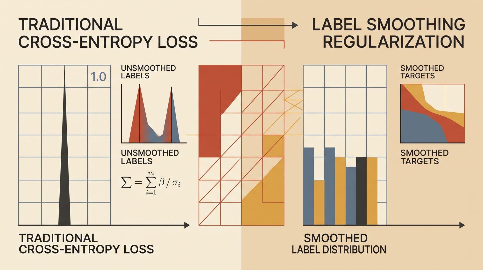
Label Smoothing Regularization: Mathematical Foundations, Maximum Entropy Dynamics, and the Regular Simplex Geometry in LLMs

In supervised classification and autoregressive language modeling, standard cross-entropy loss trains neural networks against discrete, one-hot target distributions. While intuitive, one-hot supervision creates an inherent optimization pathology: minimizing the cross-entropy objective to zero requires pushing the logit of the target class toward positive infinity while driving all competing non-target logits toward negative infinity. In deep networks, this dynamic inflates parameter norms, causes extreme prediction overconfidence, and leads to poorly calibrated probability estimates.

Label Smoothing Regularization (LSR), introduced by Szegedy et al. (2016) and adopted in foundational transformer architectures such as Vaswani et al. (2017), resolves this pathology by blending the ground-truth delta distribution with a uniform prior over the label space. Beyond empirical improvements in generalization and Expected Calibration Error (ECE), label smoothing alters the underlying loss geometry, bounds optimal logit margins, and reshapes penultimate layer representations into regular geometric simplices on the unit hypersphere.

Standard Cross-Entropy (One-Hot Target):
Ground Truth: y = [0,  0,  1.0,  0,  0]  --> Minimizing loss drives logits to ±∞

Label Smoothing Regularization (ε = 0.1, K = 5):
Target:       y = [0.02, 0.02, 0.92, 0.02, 0.02]  --> Minimizing loss bounds logits to finite margins

Mathematical Formulation of Label Smoothing

Let $x$ denote an input representation, and let $y \in \{1, \dots, K\}$ represent the ground-truth categorical label from a vocabulary or class set of size $K$ . A neural network computes unnormalized logits $z = (z_1, z_2, \dots, z_K)^T$ , which are mapped to predicted class probabilities $q(k \mid x)$ via the softmax function:

$q(k \mid x) = \frac{\exp(z_k)}{\sum_{j=1}^K \exp(z_j)}$

Under standard empirical risk minimization with hard targets, the true conditional distribution is represented as a Dirac delta (one-hot) distribution:

$p(k \mid x) = \delta_{k, y} = \begin{cases} 1 & \text{if } k = y \\ 0 & \text{if } k \neq y \end{cases}$

The standard cross-entropy loss for an individual sample is:

$\mathcal{L}_{\text{CE}}(p, q) = -\sum_{k=1}^K p(k \mid x) \log q(k \mid x) = -\log q(y \mid x) = -z_y + \log \left( \sum_{j=1}^K \exp(z_j) \right)$

The Smoothed Target Distribution

Label smoothing replaces the one-hot distribution $p(k \mid x)$ with a convex combination of the ground-truth indicator and a uniform prior distribution $u(k) = \frac{1}{K}$ over all $K$ classes, parametrized by a smoothing factor $\epsilon \in (0, 1)$ :

$p_{\epsilon}(k \mid x) = (1 - \epsilon) \delta_{k, y} + \frac{\epsilon}{K}$

Evaluating the cross-entropy under $p_{\epsilon}(k \mid x)$ yields:

$\mathcal{L}_{\text{LS}}(p_\epsilon, q) = -\sum_{k=1}^K p_{\epsilon}(k \mid x) \log q(k \mid x) = -(1 - \epsilon) \log q(y \mid x) - \frac{\epsilon}{K} \sum_{k=1}^K \log q(k \mid x)$

Expanding the formulation reveals that label smoothing decomposes into the standard cross-entropy loss and the cross-entropy between the uniform distribution $u$ and the model predictions $q$ :

$\mathcal{L}_{\text{LS}}(p_\epsilon, q) = (1 - \epsilon) \mathcal{L}_{\text{CE}}(p, q) + \epsilon \mathcal{L}_{\text{CE}}(u, q)$

Using the identity $\mathcal{L}_{\text{CE}}(u, q) = D_{\text{KL}}(u \parallel q) + H(u)$ , where $H(u) = \log K$ is the constant entropy of the uniform distribution, the loss can be expressed as:

$\mathcal{L}_{\text{LS}}(p_\epsilon, q) = (1 - \epsilon) \mathcal{L}_{\text{CE}}(p, q) + \epsilon D_{\text{KL}}(u \parallel q) + \epsilon \log K$

Minimizing the label-smoothed objective simultaneously minimizes prediction error on the true class and penalizes the Kullback-Leibler divergence between the uniform distribution and the predicted distribution, explicitly regularizing the network against sharp, degenerate output distributions.

Relationship to Maximum Entropy Regularization

The mathematical connection between label smoothing and entropy regularization was formalized by Pereyra et al. (2017) and generalized by Meister, Salesky, and Cotterell (2020).

Pereyra et al. proposed penalizing confident predictions directly by subtracting the Shannon entropy $H(q) = -\sum_{k=1}^K q(k) \log q(k)$ from the cross-entropy objective:

$\mathcal{L}_{\text{CP}}(q) = \mathcal{L}_{\text{CE}}(p, q) - \beta H(q) = \mathcal{L}_{\text{CE}}(p, q) + \beta \sum_{k=1}^K q(k) \log q(k)$

Notice the directional distinction between Confidence Penalty and Label Smoothing:

Confidence Penalty: Adds $\beta D_{\text{KL}}(q \parallel u)$ , minimizing the forward KL divergence from the model distribution to the uniform prior.
Label Smoothing: Adds $\epsilon D_{\text{KL}}(u \parallel q)$ , minimizing the reverse KL divergence from the uniform prior to the model distribution.

Because reverse KL divergence penalizes zero-probability assignments across any class (since $\frac{1}{K} \log \frac{1/K}{q(k)} \to \infty$ as $q(k) \to 0$ ), label smoothing acts as a hard barrier function that strictly prevents logits from drifting to $-\infty$ .

Logit Space Dynamics and Bounded Margin Proof

To understand how label smoothing stabilizes optimization, analyze the gradient with respect to logit $z_k$ :

$\frac{\partial \mathcal{L}_{\text{LS}}}{\partial z_k} = q(k \mid x) - p_{\epsilon}(k \mid x)$

Setting the gradient to zero demonstrates that stationary convergence occurs when the model probabilities match the smoothed target distribution exactly:

$q^*(k \mid x) = p_{\epsilon}(k \mid x) = \begin{cases} 1 - \epsilon + \frac{\epsilon}{K} = 1 - \frac{K-1}{K}\epsilon & \text{if } k = y \\ \frac{\epsilon}{K} & \text{if } k \neq y \end{cases}$

Derivation of Optimal Logit Difference

In standard cross-entropy ( $\epsilon = 0$ ), the ratio $\frac{q^(y)}{q^(k)} = \frac{1}{0} \to \infty$, requiring $z_y^* - z_k^* \to \infty$ .

Under label smoothing ( $\epsilon > 0$ ), take the ratio of softmax probabilities between target class $y$ and any non-target class $k \neq y$ :

$\frac{q^<em>(y)}{q^</em>(k)} = \frac{\exp(z_y^<em>)}{\exp(z_k^</em>)} = \exp(z_y^* - z_k^*)$

Substituting the optimal probability values:

$\exp(z_y^* - z_k^*) = \frac{1 - \frac{K-1}{K}\epsilon}{\frac{\epsilon}{K}} = \frac{K - (K-1)\epsilon}{\epsilon} = \frac{(K-1)(1 - \epsilon)}{\epsilon} + 1$

Taking the natural logarithm yields the exact analytical optimal logit difference:

$z_y^* - z_k^* = \log \left( \frac{(K-1)(1 - \epsilon)}{\epsilon} + 1 \right)$

For large vocabularies where $K \gg 1$ (such as language model tokenizers where $K \approx 32,000$ to $256,000$ ):

$z_y^* - z_k^* \approx \log \left( \frac{K(1 - \epsilon)}{\epsilon} \right) = \log K + \log \left( \frac{1 - \epsilon}{\epsilon} \right)$

This finite bound has profound implications for deep neural network training:

Parameter Norm Control: Because the maximum required logit gap is strictly bounded by a constant, gradient updates decay to zero once logits reach this margin. Weight decay is no longer fighting a diverging loss gradient, preventing runaway growth of weight matrices.
Hessian Conditioning: The maximum eigenvalue of the loss Hessian remains well-behaved, avoiding steep, ill-conditioned ravines that induce training instability in deep transformers.

Logit Gap Dynamics Comparison:
Standard Cross-Entropy:  z_y - z_k --> ∞      (Gradients stay non-zero; weights inflate)
Label Smoothing (ε=0.1): z_y - z_k = log(9K)  (Gradients vanish at target margin; weights stay bounded)

Penultimate Layer Geometry: The Regular Simplex Phenomenon

In a landmark study, Müller, Kornblith, and Hinton (NeurIPS 2019) investigated the internal representation geometry enforced by label smoothing on the penultimate layer activations $h \in \mathbb{R}^d$ .

Penultimate Layer Representation Geometry

Consider a classification layer computing logits via linear projections $z_k = w_k^T h + b_k$ . Assuming normalized weights $\|w_k\|_2 = c$ and zero bias, the squared Euclidean distance between activation $h$ and weight template $w_k$ is:

$\|h - w_k\|_2^2 = \|h\|_2^2 - 2 w_k^T h + \|w_k\|_2^2 = \|h\|_2^2 - 2 z_k + c^2$

Thus, maximizing the logit $z_k$ corresponds directly to minimizing the Euclidean distance between activation $h$ and template vector $w_k$ .

Geometric Separation: Standard CE vs. Label Smoothing

Standard Cross-Entropy ( $\epsilon = 0$ ): The network pushes activation $h$ as far as possible in the direction of $w_y$ , while pushing it away from non-target templates. Because different training examples have distinct non-target similarities, representations form diffuse, elongated clusters that spread arbitrarily along high-variance directions.
Label Smoothing ( $\epsilon > 0$ ): The network requires $h$ to maintain an exact, constant distance from target template $w_y$ , while maintaining an identical, equidistant separation from all non-target templates $w_k$ ( $k \neq y$ ).

Müller et al. proved that to satisfy this equidistant constraint simultaneously across all classes, the penultimate layer activations must collapse into dense, spherical clusters located at the vertices of a regular $(K-1)$ -simplex centered at the origin on a hypersphere.

Penultimate Layer Representation Structure:

Standard Cross-Entropy:
[Class A] ~ ~ ~ ~ (Diffuse cluster, wide variance, irregular margins to B and C)
[Class B] ~ ~ ~ ~
[Class C] ~ ~ ~ ~

Label Smoothing:
     (Class A Vertex)
          /\
         /  \
        /    \
       /      \
      /        \
(Class B) ---- (Class C)   <-- Equidistant vertices of a regular simplex on hypersphere

This structural collapse provides two distinct benefits:

Intra-Class Variance Reduction: Activations for tokens or examples belonging to the same category cluster tightly around their class center, improving linear separability.
Equidistant Inter-Class Margins: Prevents over-specialization toward spurious correlations between specific pairs of classes.

Application to Large Language Models and Sequence-to-Sequence

Label smoothing played a foundational role in the emergence of sequence-to-sequence transformers. In Attention Is All You Need (Vaswani et al., 2017), the authors trained the original Transformer model using $\epsilon_{ls} = 0.1$ .

The Perplexity vs. Generation Quality Trade-Off

In autoregressive language modeling, evaluating a label-smoothed model on validation perplexity requires careful interpretation:

$\text{PPL} = \exp \left( -\frac{1}{N} \sum_{i=1}^N \log q(y_i \mid x_{<i}) \right)$

Because label smoothing penalizes peak probabilities on ground-truth tokens (capping $q(y)$ at $1 - \frac{K-1}{K}\epsilon$ ), a model trained with label smoothing will systematically record higher (worse) validation perplexity than an identical model trained with standard cross-entropy.

However, this higher perplexity does not indicate degraded generation quality. Standard cross-entropy achieves lower perplexity by outputting overconfident, uncalibrated probability spikes. Label-smoothed models distribute probability mass across plausible synonyms and alternate token continuations, reducing repetition loops and improving beam search diversity.

Perplexity vs. Model Calibration:

Standard Cross-Entropy:
Validation Perplexity: Lower (Artificially confident on top token)
Expected Calibration Error (ECE): High (Overconfident on mistakes)
Output Entropy: Extremely low / spiky

Label Smoothing (ε = 0.1):
Validation Perplexity: Higher (Entropy floor enforced by uniform prior)
Expected Calibration Error (ECE): Low (Well-calibrated probabilities)
Output Entropy: Smooth / robust across vocabulary

The Knowledge Distillation Dilemma

While label smoothing improves calibration and standalone generalization, Müller et al. (2019) demonstrated a major theoretical and practical failure mode: models trained with label smoothing perform poorly as teachers in Knowledge Distillation.

Information Erasure in "Dark Knowledge"

Knowledge Distillation (Hinton et al., 2015) relies on "dark knowledge"—the subtle, non-zero probability structure over non-target classes generated by a teacher model. For example, when classifying an image of a BMW, a well-calibrated teacher assigns a small probability to "Audi" or "Mercedes" and near-zero probability to "Banana" or "Airplane". This relative geometry provides dense supervisory signals to student networks.

When a teacher is trained with label smoothing:

Activations collapse into equidistant vertices of a regular simplex.
The model forces all non-target logits $z_k$ ( $k \neq y$ ) to converge to identical values.
The relative semantic similarity between non-target classes is erased.

Teacher Output Probabilities on Token "Automobile":

Standard Cross-Entropy Teacher (Preserves Semantic Dark Knowledge):
P("Car") = 0.85
P("Truck") = 0.10   <-- High relative non-target probability (useful for student)
P("Bicycle") = 0.04
P("Banana") = 0.0001

Label-Smoothed Teacher (Erases Semantic Dark Knowledge):
P("Car") = 0.90
P("Truck") = 0.00033  <-- Flattened to uniform noise floor
P("Bicycle") = 0.00033
P("Banana") = 0.00033

Because all non-target classes are forced toward the uniform floor $\frac{\epsilon}{K}$ , student networks trained on soft distillation targets from a label-smoothed teacher lose the structured similarity manifold, resulting in lower downstream student accuracy compared to distilling from an unregularized teacher.

Interaction with Modern Post-Training Alignment (RLHF and DPO)

The widespread adoption of preference optimization techniques—such as Direct Preference Optimization (DPO) and Simple Preference Optimization (SimPO)—introduces additional considerations for label smoothing.

DPO parameterizes implicit reward margins using the log-likelihood ratio between the policy $\pi_\theta$ and reference model $\pi_{\text{ref}}$ :

$r(x, y) = \beta \log \frac{\pi_\theta(y \mid x)}{\pi_{\text{ref}}(y \mid x)}$

If the base reference model was pre-trained or fine-tuned with heavy label smoothing, the reference distribution $\pi_{\text{ref}}$ exhibits artificially high entropy and flattened log-probability differences. When computing log-odds ratios during alignment:

The compressed logit range reduces the dynamic resolution of the implicit reward $r(x, y)$ .
Optimization gradients on winning completions $y_w$ vs. losing completions $y_l$ become sensitive to the uniform smoothing floor, leading to unstable policy drift during long alignment runs.

Consequently, modern LLM post-training pipelines typically omit label smoothing during the final Supervised Fine-Tuning (SFT) stage preceding DPO/PPO alignment, or restrict $\epsilon$ to small values ( $\epsilon \le 0.01$ ).

PyTorch Reference Implementation

In modern deep learning frameworks, label smoothing is implemented directly inside the fused cross-entropy kernel to avoid allocating explicit $B \times S \times K$ smoothed probability tensors in GPU memory.

import torch
import torch.nn as nn
import torch.nn.functional as F

class LabelSmoothedCrossEntropy(nn.Module):
    """
    Memory-efficient fused Label Smoothed Cross Entropy Loss.
    Computes (1 - eps) * CE + eps * Uniform_CE directly from logits.
    """
    def __init__(self, epsilon: float = 0.1, ignore_index: int = -100):
        super().__init__()
        self.epsilon = epsilon
        self.ignore_index = ignore_index

    def forward(self, logits: torch.Tensor, targets: torch.Tensor) -> torch.Tensor:
        """
        Args:
            logits: (Batch, Seq_Len, Vocab_Size) or (N, Vocab_Size)
            targets: (Batch, Seq_Len) or (N,) ground-truth class indices
        """
        vocab_size = logits.size(-1)
        
        # Flatten spatial dimensions for sequence models
        logits_flat = logits.view(-1, vocab_size)
        targets_flat = targets.view(-1)
        
        # Filter masked tokens (e.g., padding or prompt tokens)
        valid_mask = targets_flat != self.ignore_index
        logits_valid = logits_flat[valid_mask]
        targets_valid = targets_flat[valid_mask]
        
        if targets_valid.numel() == 0:
            return torch.tensor(0.0, device=logits.device, requires_grad=True)
            
        # Compute log-softmax values
        log_probs = F.log_softmax(logits_valid, dim=-1)
        
        # NLL loss for ground-truth target: -log q(y)
        nll_loss = -log_probs.gather(dim=-1, index=targets_valid.unsqueeze(1)).squeeze(1)
        
        # Uniform cross-entropy: -mean(log q(k)) across vocabulary
        smooth_loss = -log_probs.mean(dim=-1)
        
        # Combined objective: (1 - eps) * NLL + eps * Smooth_Loss
        loss = (1.0 - self.epsilon) * nll_loss + self.epsilon * smooth_loss
        
        return loss.mean()

Architectural Comparison of Output Regularization Methods

Standard Cross-Entropy (One-Hot Targets):
Objective: $-\log q(y)$
Optimal Logit Gap: Infinite ( $z_y - z_k \to \infty$ )
Weight Norm Growth: Runaway inflation in the absence of aggressive weight decay
Penultimate Geometry: Elongated, high-variance clusters spreading along unconstrained directions
Distillation Utility: High (preserves subtle relative probability structure and dark knowledge)
Calibration (ECE): Poor (generates extreme overconfident probability spikes)
Label Smoothing Regularization (LSR):
Objective: $(1-\epsilon)\mathcal{L}_{\text{CE}} + \epsilon D_{\text{KL}}(u \parallel q)$
Optimal Logit Gap: Strictly bounded ( $\log \frac{(K-1)(1-\epsilon)}{\epsilon}$ )
Weight Norm Growth: Automatically bounded once gradients cut off at target margins
Penultimate Geometry: Equidistant vertices of a regular $(K-1)$ -simplex on a hypersphere
Distillation Utility: Low (erases semantic differences across non-target classes)
Calibration (ECE): Excellent (enforces smooth entropy floor across vocabulary)
Confidence Penalty (Maximum Entropy):
Objective: $\mathcal{L}_{\text{CE}} + \beta D_{\text{KL}}(q \parallel u)$
Optimal Logit Gap: Bounded via entropy gradient slope
Weight Norm Growth: Bounded by continuous entropy regularization
Penultimate Geometry: Compressed cluster variance without strict simplex formation
Distillation Utility: Medium-High (partially retains non-target relative ranking)
Calibration (ECE): Good (penalizes low-entropy output distributions)
Temperature Scaling (Post-Hoc Optimization):
Objective: Evaluated post-training via validation NLL minimization over temperature scalar $T$
Optimal Logit Gap: Modifies logit scale dynamically ( $z / T$ ) without changing training weights
Weight Norm Growth: No effect during training
Penultimate Geometry: Unchanged
Distillation Utility: High (preserves ranked probabilities while smoothing distributions)
Calibration (ECE): Excellent (optimal post-hoc recalibration technique for production inference)

Conclusion

Label Smoothing Regularization fundamentally alters the optimization landscape of classification and autoregressive modeling. By bounding the optimal logit difference to a finite value, it stops weight vector inflation, stabilizes Hessian conditioning, and collapses penultimate representations into regular simplices on the hypersphere.

While it introduces trade-offs in knowledge distillation and preference alignment, label smoothing remains a foundational technique for regularizing deep sequence architectures, preventing overconfidence, and ensuring robust calibration across large vocabularies.

Sources

Szegedy, C., Vanhoucke, V., Ioffe, S., Shlens, J., & Wojna, Z. (2016). Rethinking the Inception Architecture for Computer Vision. IEEE Conference on Computer Vision and Pattern Recognition (CVPR).
Müller, R., Kornblith, S., & Hinton, G. E. (2019). When Does Label Smoothing Help?. Advances in Neural Information Processing Systems (NeurIPS).
Pereyra, G., Tucker, G., Chorowski, J., Kaiser, Ł., & Hinton, G. (2017). Regularizing Neural Networks by Penalizing Confident Output Distributions. ICLR Workshop Track.
Meister, C., Salesky, E., & Cotterell, R. (2020). Generalized Entropy Regularization or: There’s Nothing Special about Label Smoothing. Association for Computational Linguistics (ACL).
Vaswani, A., Shazeer, N., Parmar, N., Uszkoreit, J., Jones, L., Gomez, A. N., Kaiser, Ł., & Polosukhin, I. (2017). Attention Is All You Need. Advances in Neural Information Processing Systems (NeurIPS).
Hinton, G., Vinyals, O., & Dean, J. (2015). Distilling the Knowledge in a Neural Network. NIPS Deep Learning and Representation Learning Workshop.