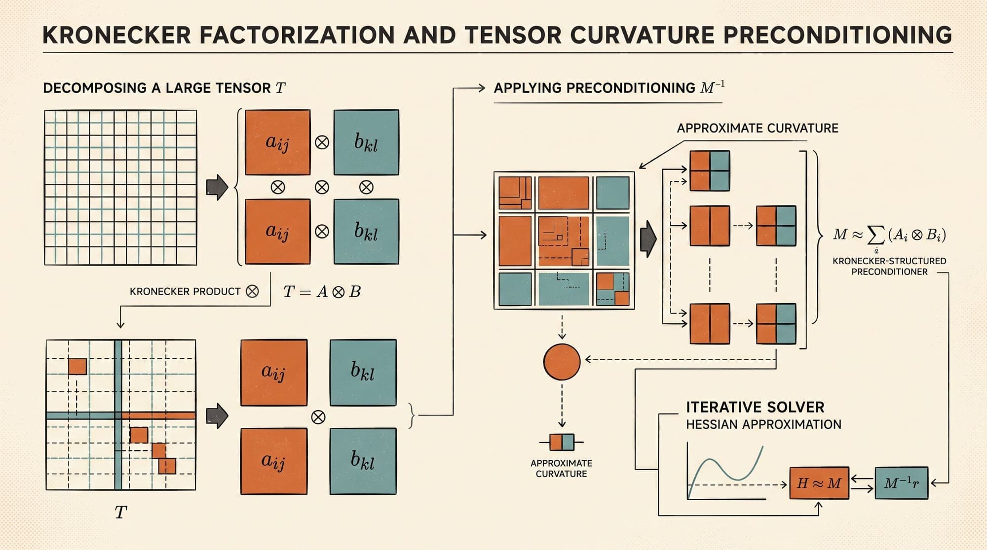
Kronecker-Factored Approximate Curvature (K-FAC) and Shampoo: How Kronecker Preconditioning Scales Second-Order Optimization

Standard deep neural network pre-training relies almost exclusively on first-order stochastic gradient methods. Optimizers such as AdamW maintain running averages of individual parameter gradients and uncentered second moments, applying a coordinate-wise diagonal preconditioner. While computationally efficient, diagonal scaling ignores off-diagonal cross-layer and intra-layer parameter correlations. When loss surfaces exhibit high anisotropy (narrow, ill-conditioned valleys with extreme curvature variation), diagonal first-order methods require thousands of micro-steps to navigate terrain that second-order methods could traverse in far fewer iterations.

Exact second-order methods, such as classical Newton-Raphson or Natural Gradient Descent, scale quadratically in memory and cubically in compute with respect to parameter count. For modern neural networks spanning billions of parameters, calculating, storing, and inverting the full Hessian or Fisher Information Matrix is intractable.

Kronecker-factored methods solve this computational barrier. By exploiting the Kronecker product structure inherent in neural network layer gradients, algorithms such as K-FAC (Martens & Grosse, 2015) and Shampoo (Gupta et al., 2018; Anil et al., 2020) approximate full-matrix curvature using compact block factors. This architecture enables tractable second-order preconditioning at scale.

1. The Second-Order Bottleneck

In standard optimization, minimizing a scalar empirical risk $L(\theta)$ over parameters $\theta \in \mathbb{R}^N$ via Newton's method employs the update rule:

$$\theta_{t+1} = \theta_t - \eta H^{-1} \nabla L(\theta_t)$$

where $H = \nabla^2 L(\theta) \in \mathbb{R}^{N \times N}$ is the Hessian matrix of second derivatives.

In probabilistic models optimized via log-likelihood objectives, Natural Gradient Descent (Amari, 1998) replaces the parameter-space Euclidean metric with the Riemannian metric tensor defined by the Fisher Information Matrix (FIM) $F$:

$$F = \mathbb{E}_{x \sim p(x), y \sim p(y|x; \theta)} \left[ \nabla_\theta \log p(y|x; \theta) \nabla_\theta \log p(y|x; \theta)^T \right]$$

For negative log-likelihood loss functions, the expected Fisher matrix is mathematically equivalent to the Generalized Gauss-Newton (GGN) matrix, providing a positive semi-definite curvature approximation that avoids negative curvature instabilities.

+-------------------------------------------------------------------------+
|                  The Second-Order Computational Ceiling                 |
+-------------------------------------------------------------------------+
|  Model Parameter Count (N)  |  Hessian/Fisher Memory  | Inversion Cost  |
|                             |  O(N^2) Elements (FP32) | O(N^3) FLOPs    |
+-----------------------------+-------------------------+-----------------+
|  100 Million (Small Model)  |  40,000 Terabytes       | ~10^24 FLOPs    |
|  1 Billion (Medium Model)   |  4 Exabytes             | ~10^27 FLOPs    |
|  70 Billion (LLM Scale)     |  19.6 Zettabytes        | ~3.4x10^32 FLOPs|
+-------------------------------------------------------------------------+

Because full-matrix representation is impossible at these dimensions, practitioners historically chose between two extremes:

1. Diagonal Approximations (Adam, RMSProp): Retain only the $N$ diagonal elements of curvature. Memory drops to $O(N)$ and inversion to $O(N)$, but all parameter cross-talk is discarded.
2. Hessian-Free / Krylov Subspace Methods: Compute Hessian-vector products $H v$ iteratively using automatic differentiation without materializing $H$ (Martens, 2010). While memory-efficient, obtaining an accurate descent direction requires dozens of conjugate gradient iterations per parameter update step, resulting in prohibitive per-iteration wall-clock overhead.

2. K-FAC: Kronecker-Factored Approximate Curvature

K-FAC (Martens & Grosse, 2015) introduces a structured structural approximation that bridges diagonal and full-matrix preconditioning. It operates on two foundational structural insights: layer-wise block diagonalization and the Kronecker decomposition of layer Fisher blocks.

The Layer Gradient Outer Product

Consider a standard fully connected layer $l$ computing activations:

$$s_l = W_l a_{l-1}, \quad a_l = \phi(s_l)$$

where $a_{l-1} \in \mathbb{R}^{d_{\text{in}}}$ is the input activation vector, $W_l \in \mathbb{R}^{d_{\text{out}} \times d_{\text{in}}}$ is the weight matrix, and $s_l \in \mathbb{R}^{d_{\text{out}}}$ is the pre-activation vector.

Let $g_l = \nabla_{s_l} L \in \mathbb{R}^{d_{\text{out}}}$ denote the loss gradient with respect to pre-activations. By the chain rule, the gradient with respect to the weight matrix $W_l$ is the outer product:

$$\nabla_{W_l} L = g_l a_{l-1}^T$$

Vectorizing this gradient using the column-stacking operator $\text{vec}(\cdot)$ yields:

$$\text{vec}(\nabla_{W_l} L) = a_{l-1} \otimes g_l$$

where $\otimes$ denotes the Kronecker product.

The Expectation Decoupling Assumption

The exact Fisher Information block $F_l \in \mathbb{R}^{(d_{\text{in}} d_{\text{out}}) \times (d_{\text{in}} d_{\text{out}})}$ corresponding to layer $l$ is the expected outer product of vectorized gradients:

$$F_l = \mathbb{E} \left[ \text{vec}(\nabla_{W_l} L) \text{vec}(\nabla_{W_l} L)^T \right] = \mathbb{E} \left[ (a_{l-1} \otimes g_l)(a_{l-1} \otimes g_l)^T \right] = \mathbb{E} \left[ (a_{l-1} a_{l-1}^T) \otimes (g_l g_l^T) \right]$$

The exact expectation of a Kronecker product couples activations and output gradients. K-FAC makes the core approximation of factoring the expectation of the product into the product of expectations:

$$\hat{F}_l = \mathbb{E} \left[ a_{l-1} a_{l-1}^T \right] \otimes \mathbb{E} \left[ g_l g_l^T \right] = A_{l-1} \otimes S_l$$

where:

• $A_{l-1} = \mathbb{E}[a_{l-1} a_{l-1}^T] \in \mathbb{R}^{d_{\text{in}} \times d_{\text{in}}}$ is the uncentered covariance matrix of incoming activations.
• $S_l = \mathbb{E}[g_l g_l^T] \in \mathbb{R}^{d_{\text{out}} \times d_{\text{out}}}$ is the uncentered covariance matrix of pre-activation derivatives.

Inversion via Kronecker Algebra

The computational advantage of K-FAC stems from the algebraic property of Kronecker products: the inverse of a Kronecker product equals the Kronecker product of the individual inverses:

$$\hat{F}_l^{-1} = (A_{l-1} \otimes S_l)^{-1} = A_{l-1}^{-1} \otimes S_l^{-1}$$

Using the standard vectorization identity $(B^T \otimes A) \text{vec}(X) = \text{vec}(A X B)$, the natural gradient update direction $\tilde{\nabla}_{W_l} L = \text{vec}^{-1}(\hat{F}_l^{-1} \text{vec}(\nabla_{W_l} L))$ simplifies directly to matrix multiplication:

$$\tilde{\nabla}_{W_l} L = S_l^{-1} (\nabla_{W_l} L) A_{l-1}^{-1}$$

+-------------------------------------------------------------------------+
|                  K-FAC Complexity Reduction (d_in x d_out)              |
+-------------------------------------------------------------------------+
|  Operation               | Full Block Matrix     | K-FAC Factorization  |
+--------------------------+-----------------------+----------------------+
|  Matrix Storage          | O(d_in^2 * d_out^2)   | O(d_in^2 + d_out^2)  |
|  Matrix Inversion        | O(d_in^3 * d_out^3)   | O(d_in^3 + d_out^3)  |
|  Preconditioning Step    | O(d_in^2 * d_out^2)   | O(d_in * d_out *     |
|                          |                       |   (d_in + d_out))    |
+-------------------------------------------------------------------------+

For a typical linear layer with $d_{\text{in}} = 4096$ and $d_{\text{out}} = 4096$:

• Exact block inversion requires inverting a $(16.7 \times 10^6) \times (16.7 \times 10^6)$ matrix, taking approximately $4.7 \times 10^{21}$ FLOPs and 1.1 petabytes of memory.
• K-FAC inverts two $4096 \times 4096$ matrices, taking approximately $1.3 \times 10^{11}$ FLOPs and 134 megabytes of memory. This represents a compute reduction exceeding 10 orders of magnitude.

Tikhonov Damping

In practice, curvature estimates require regularization to ensure positive definiteness and bound step sizes. Standard damping adds a diagonal term $(\hat{F}_l + \gamma I)^{-1}$. However, adding a diagonal directly breaks the Kronecker product factorization because $(A \otimes S + \gamma I)^{-1} \neq (A + \gamma_1 I)^{-1} \otimes (S + \gamma_2 I)^{-1}$.

K-FAC resolves this by distributing damping across factors using a scalar factor $\pi_l = \sqrt{\frac{\text{Tr}(A_{l-1}) / d_{\text{in}}}{\text{Tr}(S_l) / d_{\text{out}}}}$:

$$(A_{l-1} + \pi_l \sqrt{\gamma} I)^{-1} \otimes \left( S_l + \frac{1}{\pi_l} \sqrt{\gamma} I \right)^{-1}$$

This formulation guarantees that the Kronecker structure is strictly preserved during matrix inversion.

3. Shampoo: Preconditioned Stochastic Tensor Optimization

While K-FAC is derived from the Fisher Information Matrix in feed-forward layers, Shampoo (Gupta et al., 2018; Anil et al., 2020) generalizes full-matrix AdaGrad to arbitrary tensor parameters using multidimensional Kronecker preconditioning.

Tensor Preconditioning Formulation

For a parameter matrix $W \in \mathbb{R}^{m \times n}$ with stochastic gradient $G_t = \nabla_W L_t \in \mathbb{R}^{m \times n}$ at step $t$, full-matrix AdaGrad maintains an $(mn \times mn)$ covariance matrix $H_t = \sum_{\tau=1}^t \text{vec}(G_\tau) \text{vec}(G_\tau)^T$ and applies $H_t^{-1/2} \text{vec}(G_t)$.

Shampoo replaces the $(mn \times mn)$ tensor with two separate covariance matrices along the row and column dimensions:

$$L_t = \epsilon I_m + \sum_{\tau=1}^t G_\tau G_\tau^T \in \mathbb{R}^{m \times m}$$

$$R_t = \epsilon I_n + \sum_{\tau=1}^t G_\tau^T G_\tau \in \mathbb{R}^{n \times n}$$

The preconditioned descent direction is computed by applying symmetric fractional matrix inverse roots:

$$\Delta W_t = L_t^{-1/4} G_t R_t^{-1/4}$$

For a general order-$k$ tensor parameter $\mathcal{W} \in \mathbb{R}^{d_1 \times d_2 \times \dots \times d_k}$, Shampoo constructs $k$ preconditioner matrices $H_{(i)} \in \mathbb{R}^{d_i \times d_i}$ by contracting the outer product of gradients along all modes except mode $i$:

$$H_{(i), t} = \epsilon I_{d_i} + \sum_{\tau=1}^t G_{\tau(i)} G_{\tau(i)}^T$$

The tensor update applies the $-1/(2k)$-th power along each respective tensor mode:

$$\Delta \mathcal{W}_t = \mathcal{G}_t \times_1 H_{(1), t}^{-1/(2k)} \times_2 H_{(2), t}^{-1/(2k)} \dots \times_k H_{(k), t}^{-1/(2k)}$$

+-------------------------------------------------------------------------+
|                  Mathematical Comparison: K-FAC vs. Shampoo             |
+-------------------------------------------------------------------------+
|  Dimension               | K-FAC                     | Shampoo          |
+--------------------------+---------------------------+------------------+
|  Theoretical Origin      | Fisher Information (GGN)  | Full-Matrix      |
|                          | Natural Gradient          | AdaGrad / Tensor |
|  Factor Construction     | Activations (A) and       | Row/Column outer |
|                          | Gradients (S)             | products of G    |
|  Matrix Powers           | A^-1 and S^-1             | L^-1/4 and R^-1/4|
|                          | (Standard Inverses)       | (Inverse Roots)  |
|  Scope                   | Neural layer architectures| Arbitrary tensor |
|                          | (MLP, Conv, Attention)   | shapes           |
+-------------------------------------------------------------------------+

4. Computing Matrix Inverse Roots at Scale

Evaluating $L_t^{-1/4}$ and $R_t^{-1/4}$ efficiently and stably is the primary algorithmic challenge in Shampoo. Three main numerical approaches exist:

1. Symmetric Eigendecomposition (SVD)

Compute the spectral decomposition $L = Q \Lambda Q^T$, where $Q$ is orthogonal and $\Lambda = \text{diag}(\lambda_1, \dots, \lambda_m)$. The inverse root is:

$$L^{-1/4} = Q \Lambda^{-1/4} Q^T$$

• Pros: Exact and numerically stable even for ill-conditioned matrices.
• Cons: High computational latency on modern GPU tensor cores, which are optimized for dense GEMM (General Matrix Multiply) operations rather than sequential LAPACK tridiagonalization routines.

2. Coupled Newton-Schulz Iterations

To leverage tensor core hardware acceleration, modern distributed implementations (Anil et al., 2020) use iterative polynomial expansions that rely solely on matrix multiplications.

To compute the $p$-th inverse root $X = A^{-1/p}$ (where $p=4$ for 2D Shampoo), the coupled Newton-Schulz iteration initializes $Y_0 = A / \alpha$ and $Z_0 = I$, iterating:

$$Y_{k+1} = Y_k \left( \frac{(p+1) I - Y_k}{p} \right)$$

$$Z_{k+1} = \left( \frac{(p+1) I - Y_k}{p} \right) Z_k$$

where $\alpha$ is a scaling factor chosen to bound the spectrum inside the convergence radius ($\|Y_0 - I\| < 1$). As $k \to \infty$, $Y_k \to I$ and $Z_k \to A^{-1/p}$.

Because Newton-Schulz uses only GEMM kernels, it executes at hardware peak throughput on modern accelerator platforms.

5. Distributed Systems Architecture

Materializing and inverting preconditioners every optimization step incurs excessive communication and compute overhead. Scalable implementations, such as PyTorch Distributed Shampoo (Bernacchia et al., 2023), decouple the pipeline into asynchronous execution tiers:

+-------------------------------------------------------------------------+
|                  Distributed Asynchronous Preconditioning               |
+-------------------------------------------------------------------------+
|                                                                         |
|  [GPU Compute Stream (Every Step t)]                                    |
|      Forward Pass -> Backward Pass -> Gradient G_t                      |
|      Accumulate Statistics: L_t += G_t G_t^T,  R_t += G_t^T G_t         |
|      Apply Cached Preconditioners: \Delta W_t = P_L G_t P_R             |
|      Update Weights: W_{t+1} = W_t - \eta \Delta W_t                    |
|                                                                         |
|                          | (Every K steps, e.g. K = 50-100)             |
|                          v                                              |
|  [Asynchronous Preconditioner Engine (Host CPU or Background Stream)]    |
|      Gather Statistics Across Data-Parallel Ranks (All-Reduce / DTensor)|
|      Compute Inverse Roots: P_L = L_t^{-1/4},  P_R = R_t^{-1/4}         |
|      Send Updated Preconditioner Tensors back to Compute Engine         |
|                                                                         |
+-------------------------------------------------------------------------+

Key Engineering Optimizations:

1. Preconditioner Staleness ($K$-Step Delay): Recomputing matrix inverse roots every $K \in [20, 100]$ steps incurs negligible convergence loss while amortizing the $O(d^3)$ inversion cost over $K$ iterations.
2. Block Diagonalization of Large Tensors: For large embedding or vocabulary projection layers where $d_{\text{out}} \ge 65,536$, factoring the matrix into smaller diagonal blocks (e.g., $1024 \times 1024$ sub-matrices) bounds peak memory and compute requirements.
3. DTensor Sharding: Sharding the preconditioner state tensors across data-parallel and pipeline-parallel ranks avoids GPU out-of-memory errors during multi-node distributed training.

6. Comparison of Pre-Training Optimization Paradigms

+-------------------------------------------------------------------------------------------------------+
| Method       | Curvature Metric Captured    | Per-Step FLOP Overhead | Memory Footprint | Coordinate Invariant|
+--------------+------------------------------+------------------------+------------------+---------------------+
| SGD+Momentum | None (Euclidean)             | Low (0%)               | Low (1x params)  | No                  |
| AdamW        | Diagonal (Coordinate Variance)| Moderate (~5%)         | Medium (2x state)| No                  |
| K-FAC        | Block-Kronecker Fisher (GGN) | Moderate-High (~15-25%)| High (Covariances| Yes (Affine Layer)  |
| Shampoo      | Block-Kronecker Tensor Covar | Moderate (~10-20%)     | Medium-High      | Yes (Unitary/Linear)|
| Muon         | Orthogonal Momentum Matrix   | Low-Moderate (~5-10%)  | Medium           | Yes (Spectral)      |
+-------------------------------------------------------------------------------------------------------+

7. Current Landscape and Modern Adaptations

While first-order adaptive optimizers like AdamW remain the industry default due to implementation simplicity and minimal hyperparameter tuning, second-order Kronecker preconditioning is seeing renewed interest in frontier AI development:

1. Memory-Bandwidth Saturation: Modern GPUs provide surplus compute (TFLOPs) relative to memory bandwidth (HBM capacity and bus speed). Because K-FAC and Shampoo perform dense matrix multiplications rather than element-wise operations, their computational arithmetic intensity matches GPU hardware architecture more closely than element-wise optimizers.
2. Large-Batch Scaling: Second-order methods exhibit greater stability under very large batch sizes (hundreds of thousands to millions of tokens per step), where first-order gradient noise benefits plateau (Osawa et al., 2019).
3. Geometric Offshoots (Muon): Recent optimizer developments, such as the Muon optimizer (Jordan, 2024), adapt Shampoo's matrix-valued Newton-Schulz iterations to orthogonalize updates directly, trading off full Fisher tracking for lower computational overhead while retaining non-coordinate preconditioning dynamics.

Sources

• Martens, J., & Grosse, R. (2015). Optimizing Neural Networks with Kronecker-factored Approximate Curvature. International Conference on Machine Learning (ICML). https://arxiv.org/abs/1503.05671
• Grosse, R., & Martens, J. (2016). A Kronecker-factored Approximate Fisher Matrix for Convolutional Layers. International Conference on Machine Learning (ICML). https://arxiv.org/abs/1602.01407
• Gupta, V., Shamir, O., & Srebro, N. (2018). Shampoo: Preconditioned Stochastic Tensor Optimization. International Conference on Machine Learning (ICML). https://arxiv.org/abs/1802.09568
• Anil, R., Gupta, V., Koren, T., Regan, K., & Singer, Y. (2020). Scalable Second Order Optimization for Deep Learning. arXiv preprint. https://arxiv.org/abs/2002.09018
• Amari, S. (1998). Natural Gradient Works Efficiently in Learning. Neural Computation, 10(2), 251–276. https://doi.org/10.1162/089976698300017746
• Osawa, K., Tsuji, Y., Ueno, C., Naruse, A., Foo, C. S., & Yokota, R. (2019). Large-Scale Distributed Second-Order Optimization Using Kronecker-Factored Approximate Curvature for Deep Convolutional Neural Networks. IEEE/CVF Conference on Computer Vision and Pattern Recognition (CVPR). https://arxiv.org/abs/1811.12019
• PyTorch Distributed Shampoo Implementation. Meta Research. https://github.com/facebookresearch/optimizers