Direct Preference Optimization (DPO): Mathematical Foundations, Implicit Reward Reparameterization, Bradley-Terry Policy Derivation, and Closed-Form Alignment Dynamics

Post-training alignment is the critical bridge that transforms raw auto-regressive language models into coherent, steerable, and safe assistants. For several years, the standard approach to preference alignment relied on Reinforcement Learning from Human Feedback (RLHF) executed via Proximal Policy Optimization (PPO). While conceptually robust, PPO-based alignment requires coordinating four separate neural networks simultaneously (the active policy, value critic, reward model, and frozen reference model), generating on-policy rollouts during training, and carefully tuning hyperparameter schedules to avoid catastrophic reward hacking or policy collapse.

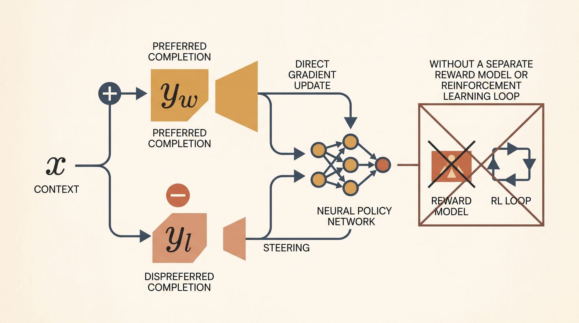
The introduction of Direct Preference Optimization (DPO) by Rafael Rafailov, Archit Sharma, Eric Mitchell, Stefano Ermon, Christopher D. Manning, and Chelsea Finn (2023) fundamentally altered post-training system design. DPO proves that the constrained reinforcement learning problem over language models can be solved exactly in closed form. By establishing a direct mathematical equivalence between the latent reward function and the optimal policy distribution, DPO eliminates the reward model and reinforcement learning loop entirely. Alignment is reduced to a single binary cross-entropy loss over static preference pairs.

This architectural explainer details the mathematical derivation of DPO from first principles, examines its gradient dynamics and implicit reward mechanics, analyzes its operational failure modes (such as length bias and likelihood displacement), and traces the evolution of the direct alignment family across modern LLM post-training pipelines.

The Classical RLHF Formulation and Its Computational Bottlenecks

To understand why DPO exists, one must first formalize the classical RLHF workflow established by Ziegler et al. (2019), Stiennon et al. (2020), and Ouyang et al. (2022).

The RLHF pipeline operates in two sequential stages:

1. Reward Model Fitting

Given a dataset of prompts $x$ and pairwise model completions $(y_w, y_l)$, where human evaluators or automated judges prefer the winning completion $y_w$ over the losing completion $y_l$, preference behavior is modeled under the Bradley-Terry (1952) probabilistic preference framework. The true latent preference probability is defined as:

$$P(y_w \succ y_l \mid x) = \sigma(r^<em>(x, y_w) - r^</em>(x, y_l)) = \frac{\exp(r^<em>(x, y_w))}{\exp(r^</em>(x, y_w)) + \exp(r^*(x, y_l))}$$

where $r^*(x, y)$ is an unobserved scalar ground-truth reward function and $\sigma(z) = \frac{1}{1 + \exp(-z)}$ is the standard logistic sigmoid function.

A parameterized reward model $r_\phi(x, y)$ is trained by minimizing the negative log-likelihood of the observed preference dataset $\mathcal{D} = \{(x^{(i)}, y_w^{(i)}, y_l^{(i)})\}_{i=1}^N$:

$$\mathcal{L}_R(r_\phi, \mathcal{D}) = -\mathbb{E}_{(x, y_w, y_l) \sim \mathcal{D}} \left[ \log \sigma \left( r_\phi(x, y_w) - r_\phi(x, y_l) \right) \right]$$

2. Reinforcement Learning Optimization

Once $r_\phi$ is frozen, the language model policy $\pi_\theta(y \mid x)$ is initialized from a supervised fine-tuned (SFT) baseline $\pi_{\text{ref}}(y \mid x)$. The policy is optimized to maximize the expected reward while penalizing divergence from $\pi_{\text{ref}}$ via Kullback-Leibler (KL) divergence:

$$\max_{\pi_\theta} \mathbb{E}_{x \sim \mathcal{D}, y \sim \pi_\theta(y \mid x)} \left[ r_\phi(x, y) \right] - \beta \mathbb{D}_{\text{KL}}\left(\pi_\theta(y \mid x) \parallel \pi_{\text{ref}}(y \mid x)\right)$$

where $\beta > 0$ is a regularization temperature controlling the penalty against policy drift away from the base model.

Practical Engineering Inefficiencies of PPO

Executing this optimization in production requires Proximal Policy Optimization (Schulman et al., 2017), which introduces severe engineering challenges:

• Four-Model GPU Memory Overhead: The training cluster must hold four distinct multi-billion parameter models in memory: the active actor policy $\pi_\theta$, the critic/value baseline $V_\psi$, the frozen reward model $r_\phi$, and the frozen reference model $\pi_{\text{ref}}$.
• On-Policy Generation Latency: During training, the actor must generate new token sequences $y \sim \pi_\theta(\cdot \mid x)$ on-policy. Generation is memory-bandwidth bound and substantially slower than forward-backward gradient passes.
• Reward Exploitation and Value Instability: Critic value head estimation errors and imperfect Generalized Advantage Estimation (GAE) often lead to optimization instability, mode collapse, or reward hacking (where the model generates nonsensical high-scoring artifacts).

Mathematical Derivation of Direct Preference Optimization

The core theoretical breakthrough of DPO is showing that the optimal solution to the KL-constrained RL objective can be derived analytically and substituted directly into the Bradley-Terry preference likelihood.

Step 1: Solving the Constrained RL Objective in Closed Form

Expanding the KL divergence in the optimization objective:

$$\max_{\pi} \mathbb{E}_{x \sim \mathcal{D}} \left[ \mathbb{E}_{y \sim \pi(y \mid x)} [r(x, y)] - \beta \sum_{y} \pi(y \mid x) \log \frac{\pi(y \mid x)}{\pi_{\text{ref}}(y \mid x)} \right]$$

This can be rewritten as:

$$\max_{\pi} \mathbb{E}_{x \sim \mathcal{D}} \left[ \sum_{y} \pi(y \mid x) \left( r(x, y) - \beta \log \frac{\pi(y \mid x)}{\pi_{\text{ref}}(y \mid x)} \right) \right]$$

Multiplying by $-\frac{1}{\beta}$ converts the maximization into an equivalent minimization:

$$\min_{\pi} \mathbb{E}_{x \sim \mathcal{D}} \left[ \sum_{y} \pi(y \mid x) \left( \log \frac{\pi(y \mid x)}{\pi_{\text{ref}}(y \mid x)} - \frac{1}{\beta} r(x, y) \right) \right]$$

We define the partition function $Z(x)$ as:

$$Z(x) = \sum_{y} \pi_{\text{ref}}(y \mid x) \exp\left( \frac{1}{\beta} r(x, y) \right)$$

This allows us to define a valid normalized probability distribution $\pi^*(y \mid x)$:

$$\pi^*(y \mid x) = \frac{1}{Z(x)} \pi_{\text{ref}}(y \mid x) \exp\left( \frac{1}{\beta} r(x, y) \right)$$

Taking the natural logarithm of both sides:

$$\log \pi^*(y \mid x) = \log \pi_{\text{ref}}(y \mid x) + \frac{1}{\beta} r(x, y) - \log Z(x)$$

Rearranging terms:

$$\frac{1}{\beta} r(x, y) = \log \frac{\pi^*(y \mid x)}{\pi_{\text{ref}}(y \mid x)} + \log Z(x)$$

Substituting this back into our minimization objective yields:

$$\min_{\pi} \mathbb{E}_{x \sim \mathcal{D}} \left[ \sum_{y} \pi(y \mid x) \left( \log \frac{\pi(y \mid x)}{\pi^*(y \mid x)} - \log Z(x) \right) \right]$$

$$\min_{\pi} \mathbb{E}_{x \sim \mathcal{D}} \left[ \mathbb{D}_{\text{KL}}\left(\pi(y \mid x) \parallel \pi^*(y \mid x)\right) - \log Z(x) \right]$$

Because $Z(x)$ depends solely on $x$, $r$, and $\pi_{\text{ref}}$ (and does not depend on the active policy $\pi$), minimizing this expression is equivalent to minimizing $\mathbb{D}_{\text{KL}}(\pi(y \mid x) \parallel \pi^*(y \mid x))$.

The minimum is achieved when the KL divergence is zero, which occurs uniquely when $\pi(y \mid x) = \pi^*(y \mid x)$. Hence, the globally optimal policy under reward $r(x, y)$ is:

$$\pi^*(y \mid x) = \frac{1}{Z(x)} \pi_{\text{ref}}(y \mid x) \exp\left(\frac{1}{\beta} r(x, y)\right)$$

Step 2: Reparameterizing the Ground-Truth Reward

Now, we invert this equation to express the latent ground-truth reward $r(x, y)$ purely in terms of the optimal policy $\pi^*$, reference policy $\pi_{\text{ref}}$, and partition function $Z(x)$:

$$r(x, y) = \beta \log \frac{\pi^*(y \mid x)}{\pi_{\text{ref}}(y \mid x)} + \beta \log Z(x)$$

This relationship holds for any optimal policy $\pi^*$. We can therefore treat any parameterized policy $\pi_\theta$ as defining an implicit reward function:

$$\hat{r}_\theta(x, y) = \beta \log \frac{\pi_\theta(y \mid x)}{\pi_{\text{ref}}(y \mid x)} + \beta \log Z(x)$$

Step 3: Canceling the Partition Function in Bradley-Terry Likelihood

The Bradley-Terry preference model depends exclusively on the difference between rewards for two completions given the same prompt $x$:

$$P(y_w \succ y_l \mid x) = \sigma\left( r(x, y_w) - r(x, y_l) \right)$$

Substituting our reparameterized implicit reward:

$$r(x, y_w) - r(x, y_l) = \left( \beta \log \frac{\pi_\theta(y_w \mid x)}{\pi_{\text{ref}}(y_w \mid x)} + \beta \log Z(x) \right) - \left( \beta \log \frac{\pi_\theta(y_l \mid x)}{\pi_{\text{ref}}(y_l \mid x)} + \beta \log Z(x) \right)$$

The intractable partition terms $\beta \log Z(x)$ cancel out exactly:

$$r(x, y_w) - r(x, y_l) = \beta \log \frac{\pi_\theta(y_w \mid x)}{\pi_{\text{ref}}(y_w \mid x)} - \beta \log \frac{\pi_\theta(y_l \mid x)}{\pi_{\text{ref}}(y_l \mid x)}$$

Step 4: The Closed-Form DPO Loss Objective

By substituting the canceled reward difference directly into the Bradley-Terry negative log-likelihood, we obtain the DPO loss function:

$$\mathcal{L}_{\text{DPO}}(\pi_\theta; \pi_{\text{ref}}) = -\mathbb{E}_{(x, y_w, y_l) \sim \mathcal{D}} \left[ \log \sigma \left( \beta \log \frac{\pi_\theta(y_w \mid x)}{\pi_{\text{ref}}(y_w \mid x)} - \beta \log \frac{\pi_\theta(y_l \mid x)}{\pi_{\text{ref}}(y_l \mid x)} \right) \right]$$

This formulation optimizes the policy directly on pairwise data using supervised cross-entropy, eliminating the separate reward model, value function, and dynamic rollouts.

Gradient Mechanics and Implicit Reward Dynamics

Analyzing the gradient of $\mathcal{L}_{\text{DPO}}$ reveals the operational mechanics governing how parameter weights are adjusted during training.

Taking the derivative with respect to $\theta$:

$$\nabla_\theta \mathcal{L}_{\text{DPO}}(\pi_\theta; \pi_{\text{ref}}) = -\beta \mathbb{E}_{(x, y_w, y_l) \sim \mathcal{D}} \left[ \underbrace{\sigma\left(\hat{r}_\theta(x, y_l) - \hat{r}_\theta(x, y_w)\right)}_{\text{Implicit Error Weight } w(x, y_w, y_l)} \cdot \underbrace{\left( \nabla_\theta \log \pi_\theta(y_w \mid x) - \nabla_\theta \log \pi_\theta(y_l \mid x) \right)}_{\text{Update Direction Vector}} \right]$$

where $\hat{r}_\theta(x, y) = \beta \log \frac{\pi_\theta(y \mid x)}{\pi_{\text{ref}}(y \mid x)}$.

The gradient decomposes into two distinct mechanisms:

1. Dynamic Error Weighting

The scalar weight $w(x, y_w, y_l) = \sigma\left(\hat{r}_\theta(x, y_l) - \hat{r}_\theta(x, y_w)\right) = 1 - \sigma\left(\hat{r}_\theta(x, y_w) - \hat{r}_\theta(x, y_l)\right)$ acts as an adaptive learning rate:

• High Error Scenarios: When the policy incorrectly assigns a higher implicit reward to the dispreferred completion ($\hat{r}_\theta(x, y_l) \gg \hat{r}_\theta(x, y_w)$), the weight approaches $1.0$, applying maximum gradient force to correct the mistake.
• Correct Ranking Scenarios: When the policy already assigns a significantly higher implicit reward to the preferred completion ($\hat{r}_\theta(x, y_w) \gg \hat{r}_\theta(x, y_l)$), the weight asymptotically approaches $0.0$, preventing over-optimization on pairs that the model has already mastered.

2. Dual Directional Updates

The directional vector $(\nabla_\theta \log \pi_\theta(y_w \mid x) - \nabla_\theta \log \pi_\theta(y_l \mid x))$ performs simultaneous push-and-pull adjustments:

• Likelihood Boosting: Pushes the policy parameters in the direction that increases the log-probability of tokens in the preferred completion $y_w$.
• Likelihood Suppression: Pulls the policy parameters in the direction that decreases the log-probability of tokens in the dispreferred completion $y_l$.

Because both completions are evaluated under log-ratio comparisons with the reference model $\pi_{\text{ref}}$, updates are strictly regularized against unconstrained probability shifts.

Practical Implementation, Hyperparameters, and Trade-offs

Deploying DPO in production requires managing several empirical properties and failure modes.

1. Temperature Hyperparameter $\beta$

The $\beta$ coefficient plays a dual role:

• It controls the strength of the implicit KL penalty relative to the reference policy.
• It acts as an inverse temperature scale on the log-probability differences.

In production fine-tuning, standard values for $\beta$ typically range from $0.01$ to $0.5$:

• High $\beta$ ($\ge 0.2$): Enforces conservative policy updates, maintaining close fidelity to the SFT base model and preventing degradation in core factual knowledge.
• Low $\beta$ ($\le 0.05$): Allows aggressive policy deviation, driving stronger adherence to stylistic or formatting preferences at the cost of increased risk of generation collapse or calibration degradation.

2. The Length Bias and Verbosity Exploitation

A well-documented vulnerability in vanilla DPO is verbosity exploitation. Because auto-regressive sequence log-probabilities are cumulative sums of individual token log-probabilities:

$$\log \pi_\theta(y \mid x) = \sum_{t=1}^{|y|} \log \pi_\theta(y_t \mid x, y_{<t})$$

longer responses have more tokens over which to accumulate log-ratio advantages if the per-token divergence is slightly positive. Consequently, models aligned with vanilla DPO often inflate generation length, producing verbose answers that mimic high-preference responses without adding factual information.

3. Likelihood Displacement on Out-of-Distribution Data

Standard DPO applies an unlikelihood penalty to all tokens in the rejected response $y_l$. However, if $y_l$ contains grammatically valid syntax, accurate factual claims, or common prefixes that overlap with $y_w$, penalizing $\log \pi_\theta(y_l \mid x)$ indiscriminately can degrade the model general language generation capabilities.

4. Reference Model Caching Optimization

During training, the reference model $\pi_{\text{ref}}$ is completely static. In production distributed training frameworks:

• If GPU memory is constrained, practitioners perform an offline pre-computation pass over the dataset to compute and store $\log \pi_{\text{ref}}(y_w \mid x)$ and $\log \pi_{\text{ref}}(y_l \mid x)$ on disk.
• This eliminates the need to hold $\pi_{\text{ref}}$ in VRAM during the backward pass, reducing the active GPU memory requirement to a single model ($\pi_\theta$) and matching standard Supervised Fine-Tuning hardware requirements.

Evolution of the Direct Alignment Family

Since the publication of DPO, several direct alignment variants have emerged to address specific structural limitations of the original formulation:

Identity Preference Optimization (IPO)

Azar et al. (2023) demonstrated that vanilla DPO can overfit when preference data contains deterministic or near-deterministic labels, driving the implicit reward difference to infinity. IPO adds a quadratic regularization term:

$$\mathcal{L}_{\text{IPO}}(\pi_\theta; \pi_{\text{ref}}) = \mathbb{E}_{(x, y_w, y_l) \sim \mathcal{D}} \left[ \left( \log \frac{\pi_\theta(y_w \mid x)}{\pi_{\text{ref}}(y_w \mid x)} - \log \frac{\pi_\theta(y_l \mid x)}{\pi_{\text{ref}}(y_l \mid x)} - \frac{1}{2\tau} \right)^2 \right]$$

This bounds policy growth and prevents log-ratio saturation.

Kahneman-Tversky Optimization (KTO)

Ethayarajh et al. (2024) adapted DPO principles to unpaired binary feedback (thumbs-up / thumbs-down signals), replacing the Bradley-Terry pairwise preference utility with Kahneman-Tversky prospect theory value functions.

Simple Preference Optimization (SimPO)

Meng et al. (2024) eliminated the reference model $\pi_{\text{ref}}$ entirely by introducing length-normalized sequence log-probabilities and an explicit target reward margin $\gamma$:

$$\mathcal{L}_{\text{SimPO}}(\pi_\theta) = -\mathbb{E}_{(x, y_w, y_l) \sim \mathcal{D}} \left[ \log \sigma \left( \frac{\beta}{|y_w|} \log \pi_\theta(y_w \mid x) - \frac{\beta}{|y_l|} \log \pi_\theta(y_l \mid x) - \gamma \right) \right]$$

SimPO prevents length exploitation while simplifying memory footprint to a single reference-free policy.

Contrastive Preference Optimization (CPO)

Xu et al. (2024) targeted machine translation and constrained generation tasks by pairing DPO implicit reward differences with explicit supervised maximum likelihood regularization, preventing out-of-distribution quality collapse.

Online and Iterative DPO

While vanilla DPO is strictly offline (training on static preference pairs), Xiong et al. (2023) and Calandriello et al. (2024) introduced iterative DPO. By generating new candidate completions on-policy at regular intervals, scoring them with an external judge or verified reward model, and updating the reference policy $\pi_{\text{ref}}$, iterative DPO bridges the gap between offline simplicity and on-policy exploration.

Architectural Comparison Across Post-Training Alignment Methods

The operational differences across major post-training alignment frameworks reflect contrasting trade-offs between memory overhead, training stability, and mathematical design:

• PPO (Proximal Policy Optimization): Requires 4 models (Actor, Critic, Reward, Reference). Operates on-policy with high training instability, high VRAM requirements, and moderate sample efficiency.
• DPO (Direct Preference Optimization): Requires 2 models (Policy and Reference; reference can be pre-computed). Operates offline with high stability, low-to-medium VRAM requirements, and high sample efficiency.
• IPO (Identity Preference Optimization): Requires 2 models. Operates offline with quadratic regularized loss, preventing overconfidence and gradient vanishing on clean datasets.
• SimPO (Simple Preference Optimization): Requires 1 model (Reference-free). Operates offline with length-normalized margin loss, minimizing VRAM overhead while resisting verbosity hacking.
• GRPO (Group Relative Policy Optimization): Requires 2 models (Actor and Reference). Uses critic-free group reward normalization for verifiable reasoning domains without a value network.

Summary and Editorial Assessment

Direct Preference Optimization represents a decisive paradigm shift in post-training machine learning. By establishing that language models are implicitly parameterizing their own reward functions, DPO eliminated the fragile multi-stage RL infrastructure previously required to align generative systems.

While nuances around length bias, hyperparameter calibration, and off-policy distribution shifts require active mitigation in production pipelines, the closed-form simplicity of DPO has established it as the architectural baseline for open-weight and frontier post-training workflows alike.

Sources

• Direct Preference Optimization: Your Language Model is Secretly a Reward Model (Rafailov et al., 2023)
• Rank Analysis of Incomplete Block Designs: I. The Method of Paired Comparisons (Bradley & Terry, 1952)
• Fine-Tuning Language Models from Human Preferences (Ziegler et al., 2019)
• Learning to Summarize from Human Feedback (Stiennon et al., 2020)
• Training Language Models to Follow Instructions with Human Feedback (Ouyang et al., 2022)
• Proximal Policy Optimization Algorithms (Schulman et al., 2017)
• A General Theoretical Paradigm to Understand Learning from Human Preferences (Azar et al., 2023 - IPO)
• KTO: Model Alignment as Prospect Theoretic Optimization (Ethayarajh et al., 2024)
• SimPO: Simple Preference Optimization with a Reference-Free Objective (Meng et al., 2024)
• Contrastive Preference Optimization for Out-of-Distribution Alignment (Xu et al., 2024)
• Iterative Preference Learning from Human Feedback: Bridging Theory and Practice (Xiong et al., 2023)