Diffusion Transformers (DiT): How Patchification and adaLN-Zero Replaced U-Nets in Generative AI

Generative visual models relied for years on convolutional U-Net architectures to execute iterative denoising. From Denoising Diffusion Probabilistic Models (DDPM) and Ablated Diffusion Models (ADM) to Latent Diffusion Models (LDMs) behind Stable Diffusion, convolutional backbones served as the default engine for image synthesis. While convolutional inductive biases provided translation equivariance and local spatial hierarchies, they imposed architectural rigidities that resisted compute scaling at large parameter volumes.

The publication of Scalable Diffusion Models with Transformers by William Peebles and Saining Xie (ICCV 2023) fundamentally altered that trajectory. By replacing the convolutional U-Net backbone with a Vision Transformer (ViT) operating over latent image patches, the Diffusion Transformer (DiT) demonstrated that generative image quality scales predictably with compute. The architectural blueprint established by DiT now underpins state-of-the-art visual generation systems, including OpenAI Sora, Black Forest Labs Flux, Stability AI Stable Diffusion 3, and Alibaba Wan 2.1.

The Limitations of Convolutional U-Nets

Convolutional U-Nets process continuous feature maps through downsampling encoder stages, a low-resolution bottleneck, and upsampling decoder stages with skip connections. This structure was designed for semantic segmentation and pixel-level dense prediction. When repurposed as score-matching networks in diffusion models, several structural bottlenecks emerged:

1. Rigid Architectural Coupling: In a U-Net, modifying capacity involves tuning channel multipliers across asymmetric resolution tiers (such as 64, 128, 256, and 512 channels across 1x, 2x, 4x, and 8x downsampling). This complicates scaling analysis and creates hardware underutilization on tensor cores optimized for uniform matrix multiplications.
2. Asymmetric Conditioning Injection: Timestep and context embeddings must be injected separately into residual blocks and cross-attention layers at multiple distinct spatial resolutions, creating uneven representational dynamics across the network.
3. Sub-Optimal Long-Range Context: Downsampling convolutions compress spatial context hierarchically, but cannot model arbitrary global dependencies across distant pixel regions without deep stacks of spatial attention layers.

Standard Transformers, by contrast, operate on flattened token sequences via uniform multi-head self-attention and point-wise feed-forward networks (FFNs). Scaling a Transformer requires adjusting three uniform hyperparameters: depth (number of layers $L$), width (hidden dimension $d$), and attention heads ($H$).

Patchification and Latent Tokenization

DiT operates within the continuous latent space of a pre-trained Variational Autoencoder (VAE). Operating in latent space rather than pixel space reduces spatial dimensionality by a factor of 8 (from $256 \times 256 \times 3$ RGB pixels to a $32 \times 32 \times 4$ latent tensor $z$), eliminating high-frequency noise and lowering computational overhead.

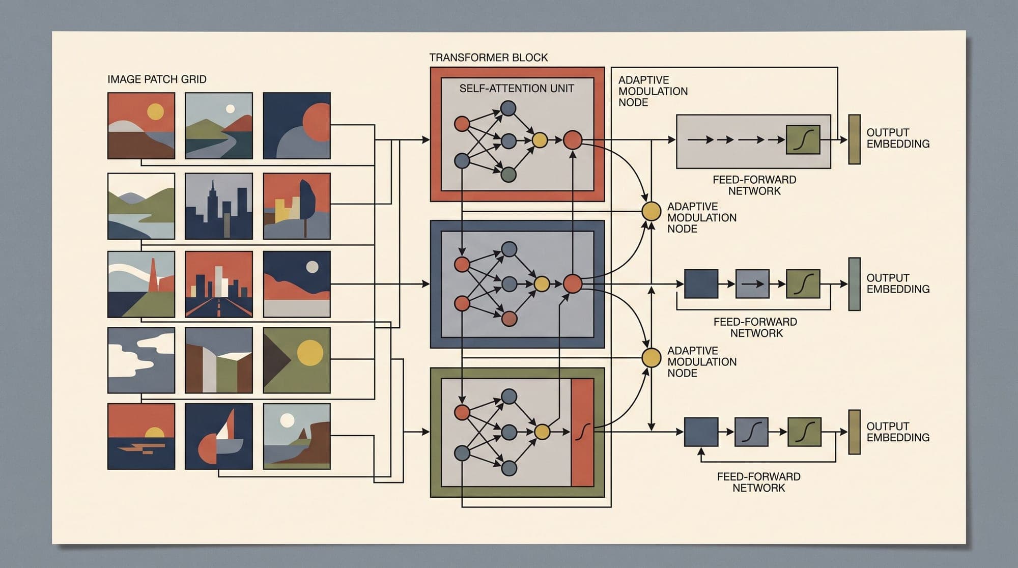
To ingest the spatial latent map into a standard Transformer, DiT uses patchification:

1. A latent representation $z \in \mathbb{R}^{H \times W \times C}$ is partitioned into a spatial grid of non-overlapping patches of spatial size $p \times p$.
2. The total number of tokens generated is $T = \left(\frac{H}{p}\right) \times \left(\frac{W}{p}\right)$.
3. Each patch of shape $p \times p \times C$ is linearly projected into a vector of hidden dimension $d$.
4. Standard 2D sinusoidal or learned positional embeddings are added to each token to preserve spatial coordinates:

$$x_0 = \text{Linear}(\text{Flatten}(\text{Patch}_{i,j})) + E_{\text{pos}}(i, j)$$

For a $32 \times 32$ latent map with patch size $p = 2$, the sequence length is $T = (32/2) \times (32/2) = 256$ tokens. With patch size $p = 4$, the sequence length drops to $T = (32/4) \times (32/4) = 64$ tokens. Decreasing patch size increases the sequence length quadratically, driving up GFLOPs without altering model parameter count.

Conditioning Paradigms: Why adaLN-Zero Won

Diffusion models require external conditioning signals at every denoising step, primarily the continuous diffusion timestep $t$ and optional context vectors $y$ (such as class labels or text prompt embeddings). Peebles and Xie systematically evaluated four conditioning architectures:

Conditioning Variants in Diffusion Transformers:
1. In-Context Conditioning:    [ t_emb | y_emb | x_1 | x_2 | ... | x_T ] -> Self-Attention
2. Cross-Attention:            Self-Attention(x) -> Cross-Attention(x, [t, y]) -> FFN(x)
3. Standard adaLN:             Scale/Shift LayerNorm parameters predicted via MLP(t, y)
4. adaLN-Zero:                 adaLN + Zero-Initialized residual gating on Attention and FFN

1. In-Context Conditioning: Timestep and class embeddings are prepended as two additional tokens to the sequence, yielding an input of length $T+2$. Standard ViT self-attention processes the full sequence. While adding negligible compute, this mechanism performed worst in empirical evaluations (FID 42.4 on DiT-XL/2 at 400K steps).
2. Cross-Attention Block: The token sequence passes through self-attention, followed by a dedicated multi-head cross-attention layer that queries the concatenated conditioning embedding $(t, y)$, followed by an FFN. This mirrors Stable Diffusion U-Nets. While effective (FID 26.3), it added roughly 15% computational overhead per block.
3. Adaptive Layer Normalization (adaLN): Standard LayerNorm applies fixed, learned affine parameters: $\text{LN}(x) = \gamma \odot \hat{x} + \beta$. In adaLN, the scale $\gamma$ and shift $\beta$ parameters are dynamically computed for each sample from the conditioning vector $c = \text{Embed}(t) + \text{Embed}(y)$:

$$\text{adaLN}(x, c) = \gamma(c) \odot \left(\frac{x - \mu}{\sigma}\right) + \beta(c)$$

1. Adaptive Layer Normalization with Zero-Initialization (adaLN-Zero): The optimal design extends adaLN by predicting six modulation parameters per block and introducing dimension-wise residual scaling factors initialized to zero.

Mathematical Mechanics of adaLN-Zero

In an adaLN-Zero transformer block, a shared conditioning vector $c$ is mapped via a single multi-layer perceptron (MLP) into six modulation vectors:

$$\left(\gamma_1, \beta_1, \alpha_1, \gamma_2, \beta_2, \alpha_2\right) = \text{MLP}(c)$$

where each parameter vector has dimension $d$ matching the hidden size of the transformer block.

The forward pass of the $l$-th DiT block executes in two sub-steps:

1. Multi-Head Self-Attention Sub-Layer

The input token representations $x$ are normalized and modulated by $\gamma_1$ and $\beta_1$, passed through standard multi-head self-attention (MHA), scaled element-wise by the gating parameter $\alpha_1$, and added back to the residual stream:

$$x' = x + \alpha_1 \odot \text{MHA}\left(\gamma_1 \odot \text{LN}(x) + \beta_1\right)$$

2. Point-Wise Feed-Forward Sub-Layer

The intermediate activation $x'$ is normalized and modulated by $\gamma_2$ and $\beta_2$, passed through the multi-layer feed-forward network (FFN), scaled element-wise by $\alpha_2$, and added back to the residual stream:

$$x_{\text{out}} = x' + \alpha_2 \odot \text{FFN}\left(\gamma_2 \odot \text{LN}(x') + \beta_2\right)$$

The Zero-Initialization Property

In standard deep transformers, training stability requires warmup schedules and careful normalization placement to prevent exploding gradients. adaLN-Zero solves this by initializing the final linear projection of the conditioning MLP to all zeros:

$$\alpha_1 = 0, \quad \alpha_2 = 0, \quad \gamma_1 = 0, \quad \gamma_2 = 0, \quad \beta_1 = 0, \quad \beta_2 = 0$$

At step zero of training, before any weight updates occur:

$$x' = x + 0 \odot \text{MHA}(\dots) = x$$ $$x_{\text{out}} = x' + 0 \odot \text{FFN}(\dots) = x' = x$$

Every DiT block acts as a pure identity mapping at initialization. Signals propagate unchanged through arbitrary network depth without attenuation or explosive growth, allowing models with 28 or more layers (such as DiT-XL) to train stably from scratch without gradient instability.

Compute Scaling and Empirical Scaling Laws

The defining contribution of the DiT architecture was formalizing scaling laws for generative diffusion models. Forward-pass computational complexity is measured directly in GigaFLOPs (GFLOPs).

Peebles and Xie defined four standard model capacity tiers:

• DiT-S (Small): 12 layers, hidden size 384, 6 attention heads, 33M parameters.
• DiT-B (Base): 12 layers, hidden size 768, 12 attention heads, 130M parameters.
• DiT-L (Large): 24 layers, hidden size 1024, 16 attention heads, 458M parameters.
• DiT-XL (Extra Large): 28 layers, hidden size 1152, 16 attention heads, 675M parameters.

Each model size was evaluated across three patch sizes: $p \in \{8, 4, 2\}$.

Model Complexity vs. Patch Size (Forward Pass GFLOPs at 256x256 resolution):
-----------------------------------------------------------------------------
Configuration | Patch Size p | Sequence Length T | GFLOPs / Step | Parameters
-----------------------------------------------------------------------------
DiT-S/8       | 8            | 16                | 0.4           | 33M
DiT-S/4       | 4            | 64                | 1.6           | 33M
DiT-S/2       | 2            | 256               | 6.1           | 33M
DiT-B/8       | 8            | 16                | 1.5           | 130M
DiT-B/4       | 4            | 64                | 5.8           | 130M
DiT-B/2       | 2            | 256               | 23.0          | 130M
DiT-L/8       | 8            | 16                | 5.3           | 458M
DiT-L/4       | 4            | 64                | 21.0          | 458M
DiT-L/2       | 2            | 256               | 80.7          | 458M
DiT-XL/8      | 8            | 16                | 7.8           | 675M
DiT-XL/4      | 4            | 64                | 31.0          | 675M
DiT-XL/2      | 2            | 256               | 118.6         | 675M
-----------------------------------------------------------------------------

Key Scaling Observations

1. Patch Size Dominates Efficiency: Decreasing patch size $p$ from 8 to 2 yields a larger quality improvement (lower Fréchet Inception Distance, or FID) than increasing model parameters from DiT-S to DiT-XL at a constant patch size. For instance, DiT-S/2 (6.1 GFLOPs, 33M params) consistently outperformed DiT-XL/8 (7.8 GFLOPs, 675M params) despite having 20x fewer parameters.
2. Predictable Power-Law Trajectory: When plotting FID against total training compute (Training GFLOPs = Forward GFLOPs $\times$ Batch Size $\times$ Training Steps), DiT exhibits a strict power-law relationship. Higher compute investment translates monotonically into lower FID and higher visual fidelity.
3. State-of-the-Art Benchmarks: The largest variant, DiT-XL/2 (with classifier-free guidance), achieved an ImageNet $256 \times 256$ class-conditional FID of 2.27, outperforming all prior diffusion models including ADM (2.92) and LDM-4 (3.60).

Architectural Descendants: MM-DiT, Flux, and 3D Spatio-Temporal DiTs

The core mechanics of DiT have evolved into several specialized architectures across modern multimodal and video foundation models:

1. Multimodal Diffusion Transformers (MM-DiT)

Introduced in Stable Diffusion 3 (Esser et al., 2024), MM-DiT processes visual tokens and text prompt tokens through separate sets of transformer weights for their respective modalities. At the attention stage, queries, keys, and values from text and image streams are concatenated, enabling bidirectional cross-modal attention without enforcing identical representation spaces for visual latents and textual semantics.

2. Dual-Stream to Single-Stream Architectures (Flux.1)

Developed by Black Forest Labs, Flux.1 adopts a hybrid architecture. The initial transformer layers maintain separate weights for text and image modalities (dual-stream blocks), allowing modality-specific conditioning. Later layers fuse into single-stream blocks where visual and textual tokens share unified feed-forward networks and self-attention projections, maximizing parameter reuse and representational depth.

3. 3D Spatio-Temporal DiTs for Video Generation

In video foundation models such as OpenAI Sora and Alibaba Wan 2.1, the 2D patchification operator is generalized to a 3D spatio-temporal tubelet extraction operator. A video latent tensor $z \in \mathbb{R}^{T \times H \times W \times C}$ is sliced into 3D spacetime patches ($p_t \times p_h \times p_w$), projected into 1D token sequences, and indexed using 3D Rotary Position Embeddings (3D-RoPE). This formulation treats video synthesis as sequence modeling over 3D spacetime grids, unifying image and video generation under a single transformer backbone.

Summary

The transition from convolutional U-Nets to Diffusion Transformers shifted generative modeling from manual architectural tuning to standard Transformer compute scaling. By pairing spatial latent patchification with adaLN-Zero modulation, DiT provided an architecture that scales with compute, trains with numerical stability, and interfaces naturally with multimodal token sequences.

Sources

• Peebles, W., & Xie, S. (2023). Scalable Diffusion Models with Transformers. Proceedings of the IEEE/CVF International Conference on Computer Vision (ICCV), 4172-4182.
• Esser, P., Kulal, S., Blattmann, A., Entezari, R., Müller, J., Saini, H., ... & Rombach, R. (2024). Scaling Rectified Flow Transformers for High-Resolution Image Synthesis. arXiv preprint arXiv:2403.03206.
• Rombach, R., Blattmann, A., Lorenz, D., Esser, P., & Ommer, B. (2022). High-Resolution Image Synthesis with Latent Diffusion Models. Proceedings of the IEEE/CVF Conference on Computer Vision and Pattern Recognition (CVPR), 10684-10695.
• Dhariwal, P., & Nichol, A. (2021). Diffusion Models Beat GANs on Image Synthesis. Advances in Neural Information Processing Systems (NeurIPS), 34, 8780-8794.