Deep Double Descent: Why Overparameterization Defies the Classical Bias-Variance Trade-Off

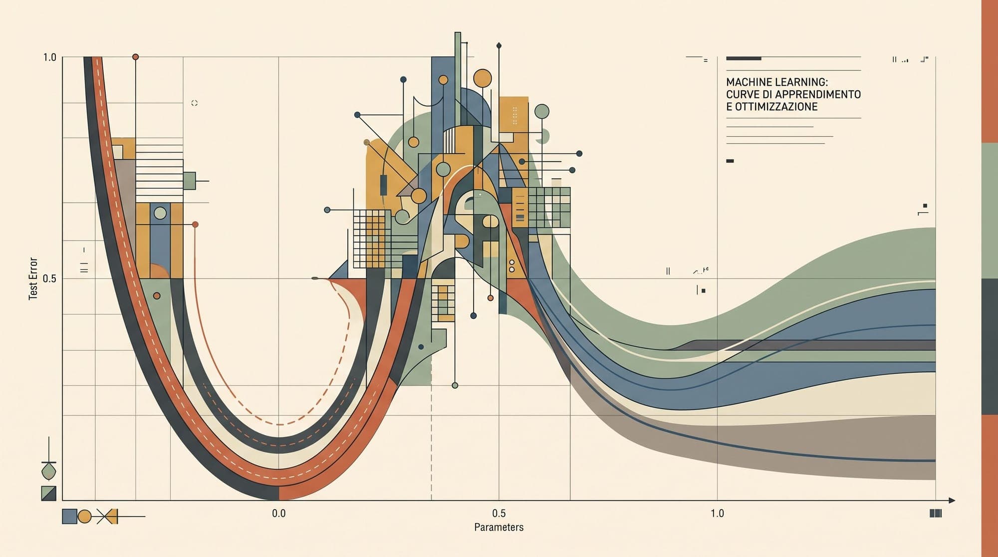
For decades, statistical learning theory rested on a foundational tenet: the bias-variance trade-off. According to classical machine learning textbooks, increasing model capacity reduces bias on the training set but inevitably inflates variance on unseen test data. The resulting risk curve forms a familiar U-shape: underfitting on the left, an optimal capacity in the center, and severe overfitting on the right.

Modern deep learning and large language models (LLMs) fundamentally contradicted this doctrine. Frontier transformers contain hundreds of billions of parameters, exceeding their token count or sample dimensionality by orders of magnitude, yet their generalization performance improves monotonically with scale.

In 2019, seminal work by Mikhail Belkin et al. and Preetum Nakkiran et al. resolved this apparent paradox by introducing the double descent risk curve. This framework demonstrates that the classical U-shaped curve describes only the underparameterized regime. As capacity continues to expand past the "interpolation threshold" (the point where a model can perfectly fit all training samples), test error experiences a temporary peak, followed by a second descent toward superior generalization.

1. The Classical View vs. Modern Practice

In classical statistical learning, total expected prediction error decomposes into three additive terms:

$$\mathbb{E}[(y - \hat{f}(x))^2] = \text{Bias}[\hat{f}(x)]^2 + \text{Var}[\hat{f}(x)] + \sigma^2$$

• Bias: The approximation error resulting from simplifying assumptions in the model family.
• Variance: The sensitivity of the estimated function to fluctuations in the specific training dataset drawn.
• Irreducible Error ($\sigma^2$): The intrinsic noise floor of the data-generating distribution.

Classical theory dictates that as model complexity $P$ approaches the sample size $N$, variance grows rapidly. Fitting noisy data points with zero residual error was widely believed to yield erratic, oscillating functions that fail catastrophically out of sample.

However, modern deep neural networks routinely achieve near-zero training loss while delivering state-of-the-art test accuracy. Belkin and colleagues proved that classical learning theory and modern overparameterized practice are two halves of a single unified performance curve.

2. The Three Regimes of the Unified Risk Curve

The double descent curve partitions the capacity spectrum into three distinct operating regimes:

Regime 1: Underparameterized ($P < N$)

In this classical domain, the model lacks sufficient parameters to fit the training set with zero error. Increasing capacity reduces bias faster than it increases variance, leading to decreasing test error until reaching an initial local minimum. As parameter count continues toward $N$, variance begins to dominate, driving test error upward.

Regime 2: The Interpolation Threshold ($P \approx N$)

At the critical boundary where effective parameter capacity matches the degrees of freedom required to fit all training points, the model is barely able to interpolate the dataset. Because exactly one or very few parameter configurations can achieve zero training error, the optimization algorithm is constrained to fit both true signal and noise with extreme sensitivity. This induces an explosion in model variance, producing a prominent peak in generalization error.

Regime 3: Overparameterized ($P \gg N$)

Once parameters far exceed the interpolation requirement, the optimization landscape undergoes a structural transition. An infinite manifold of parameter configurations now achieves zero training error (an interpolating subspace). Optimization algorithms like stochastic gradient descent (SGD) and Adam select solutions with minimal parameter norm or maximal margin. As capacity expands further, the optimization process gains additional degrees of freedom to select smoother, lower-norm interpolants, driving test error down in a second descent.

3. Mathematical Mechanism: Condition Numbers and Minimum-Norm Interpolants

The mathematical origin of double descent can be illustrated directly in high-dimensional linear regression, analyzed extensively by Hastie et al. (2019) and Bartlett et al. (2020).

Consider a dataset with $N$ samples and $P$ features, represented by feature matrix $\mathbf{X} \in \mathbb{R}^{N \times P}$ and target vector $\mathbf{y} \in \mathbb{R}^N$.

At the Interpolation Threshold ($P = N$)

The least-squares estimator computes:

$$\hat{\beta} = (\mathbf{X}^T \mathbf{X})^{-1} \mathbf{X}^T \mathbf{y}$$

As $P \to N$, the sample covariance matrix $\mathbf{X}^T \mathbf{X}$ becomes ill-conditioned. Its smallest singular value $\sigma_{\min}(\mathbf{X})$ approaches zero. The variance term scales inversely with $\sigma_{\min}^2$:

$$\text{Var}(\hat{\beta}) \propto \text{Tr}((\mathbf{X}^T \mathbf{X})^{-1}) \approx \sum_{i=1}^{\min(N, P)} \frac{1}{\sigma_i^2}$$

When $\sigma_{\min} \to 0$, the trace diverges, causing parameter magnitudes to explode to fit marginal noise points. The resulting predictor exhibits violent oscillations between data points.

In the Overparameterized Regime ($P > N$)

When $P > N$, $\mathbf{X}^T \mathbf{X}$ is singular, and the linear system $\mathbf{X}\beta = \mathbf{y}$ is underdetermined. Standard gradient descent initialized at zero converges to the Moore-Penrose pseudoinverse solution:

$$\hat{\beta} = \mathbf{X}^T (\mathbf{X} \mathbf{X}^T)^{-1} \mathbf{y} = \arg\min_{\beta} \|\beta\|_2 \quad \text{subject to} \quad \mathbf{X}\beta = \mathbf{y}$$

In this regime, the inverted matrix is the Gram matrix $\mathbf{K} = \mathbf{X} \mathbf{X}^T \in \mathbb{R}^{N \times N}$. As $P$ grows relative to $N$, the singular values of $\mathbf{X}\mathbf{X}^T$ spread out and move away from zero according to Marchenko-Pastur spectral distribution laws. The minimal $\ell_2$-norm interpolant distributes predictive weight evenly across redundant latent dimensions, suppressing variance and restoring smooth global interpolation.

4. The Three Manifestations of Deep Double Descent

In their comprehensive empirical study across CNNs, ResNets, and Transformers, Nakkiran et al. (2019) proved that double descent manifests across three operational dimensions:

1. Model-Wise Double Descent

Holding dataset size and training duration constant, varying network width or layer count causes test error to trace the classic double-descent trajectory. The peak occurs precisely at the capacity where the network transitions from non-zero training error to 0% empirical training error.

2. Sample-Wise Double Descent

Holding model architecture fixed and increasing the number of training samples $N$ can paradoxically degrade test performance when $N$ expands toward the model capacity $P$. Expanding data from an overparameterized regime into the critical threshold forces the model to struggle for interpolation, spiking variance until sample size grows large enough to place the model safely into the underparameterized regime.

3. Epoch-Wise Double Descent

Holding architecture and dataset fixed, training a model of intermediate capacity for an extended number of epochs exhibits a temporary surge in test error before recovering. During early epochs, implicit regularization keeps parameter norms small. As optimization approaches zero training loss on difficult or noisy examples, parameter norms expand rapidly (the variance peak), before gradient dynamics settle into flatter, lower-norm minima. This phenomenon is closely related to the delayed generalization dynamics observed in grokking.

5. Double Descent in Transformers and Modern LLMs

Language models exhibit distinct manifestations of double descent during pre-training and fine-tuning:

Pre-Training Scaling Laws

In frontier LLM pre-training, empirical scaling formulations established by Kaplan et al. (2020) and refined by Hoffmann et al. (2022) show continuous, monotonic power-law improvements in cross-entropy loss:

$$L(N, D) = \left(\frac{N_c}{N}\right)^{\alpha_N} + \left(\frac{D_c}{D}\right)^{\alpha_D}$$

Why do frontier pre-training runs avoid double-descent loss spikes?

• Extreme Overparameterization: Large models with 7B to 400B parameters operate far to the right of the interpolation threshold for any local batch sequence.
• Infinite Data Streams: Pre-training on trillions of tokens means models rarely cycle through identical data points repeatedly, preventing unregularized overfitting to specific sample noise.
• Optimizers with Weight Decay: Standard pre-training recipes utilize AdamW with decoupled weight decay ($\lambda \in [0.01, 0.1]$), which explicitly penalizes large $\ell_2$ parameter norms and suppresses variance divergence.

Fine-Tuning and Domain Adaptation Risks

The critical double-descent regime re-emerges during task-specific fine-tuning. When fine-tuning moderate-sized models (e.g., 1B to 7B parameters) on small specialized datasets (1,000 to 50,000 examples) without adequate regularization:

• Full-parameter fine-tuning easily hits the interpolation threshold, leading to catastrophic forgetting and test degradation.
• Parameter-efficient techniques such as LoRA Hu et al. (2021) constrain trainable rank $r$, effectively bounding model capacity $P$ well below the critical variance explosion threshold.

6. Engineering Implications and Practical Mitigations

Understanding double descent provides actionable principles for LLM practitioners:

• Small Dataset Fine-Tuning: When parameter count matches sample degrees of freedom, use low-rank adaptation (LoRA/DoRA) or freeze backbone layers to avoid the $P \approx N$ peak.
• Noisy Training Corpora: Label and target noise drastically inflates the interpolation error peak. Apply aggressive data filtering, including deduplication, heuristic cleaning, and quality classifiers.
• Intermediate Model Sizing: When training models near capacity limits without regularization, tune AdamW weight decay ($\lambda$) to smoothly bridge the interpolation threshold.
• Training Duration Tuning: In situations where epoch-wise double descent causes temporary evaluation dips, avoid terminating training prematurely during initial validation error spikes if training loss is still contracting.

As demonstrated by Nakkiran et al., optimal $\ell_2$ regularization eliminates the double descent peak entirely, transforming the jagged trajectory into a monotonic curve that matches the envelope of best test performance.

Summary

Double descent resolves the apparent conflict between classical statistical theory and modern deep learning. Rather than indicating that bigger models overfit, learning theory proves that severe overfitting is a localized pathology of the interpolation boundary. By scaling model capacity deep into the overparameterized regime, neural networks leverage excess dimensions to discover smoother, lower-norm representations that generalize with exceptional fidelity.

Sources

• Belkin, M., Hsu, D., Ma, S., & Mandal, S. (2019). Reconciling modern machine-learning practice and the classical bias-variance trade-off. Proceedings of the National Academy of Sciences (PNAS), 116(32), 15849-15854.
• Nakkiran, P., Kaplun, G., Bansal, Y., Yang, T., Barak, B., & Sutskever, I. (2019). Deep Double Descent: Where Bigger Models and More Data Hurt. International Conference on Learning Representations (ICLR).
• Hastie, T., Montanari, A., Rosset, S., & Tibshirani, R. J. (2019). Surprises in High-Dimensional Empirical Risk Minimization: A Ridge and Curvature Perspective. arXiv preprint arXiv:1903.11247.
• Bartlett, P. L., Long, P. M., Lugosi, G., & Tsigler, A. (2020). Benign Overfitting in Linear Regression. Proceedings of the National Academy of Sciences, 117(48), 30063-30070.
• Kaplan, J., McCandlish, S., Henighan, T., Brown, T. B., Chess, B., Child, R., Gray, S., Radford, A., Wu, J., & Amodei, D. (2020). Scaling Laws for Neural Language Models. arXiv preprint arXiv:2001.08361.
• Hoffmann, J., Borgeaud, S., Mensch, A., Buchatskaya, E., Cai, T., Rutherford, E., de Las Casas, D., Hendricks, L. A., Welbl, J., Clark, A., Hennigan, T., Noland, E., Millican, K., van den Driessche, G., Damoc, B., Guy, A., Osindero, S., Simonyan, K., Elsen, E., Rae, J. W., Vinyals, O., & Sifre, L. (2022). Training Compute-Optimal Large Language Models. arXiv preprint arXiv:2203.15556.
• Power, A., Burda, Y., Edwards, H., Babuschkin, I., & Sutskever, I. (2022). Grokking: Generalization Beyond Overfitting on Small Algorithmic Datasets. arXiv preprint arXiv:2201.02177.
• Hu, E. J., Shen, Y., Wallis, P., Allen-Zhu, Z., Li, Y., Wang, S., Wang, L., & Chen, W. (2021). LoRA: Low-Rank Adaptation of Large Language Models. International Conference on Learning Representations (ICLR).