CUDA Graph Capture in Production LLM Serving: Dynamic Batch Bucketing, Static Memory Pooling, and Kernel Launch Elimination

In high-throughput large language model serving, the autoregressive generation (decode) phase presents an operational bottleneck distinct from prefill processing. While prefill computation is dominated by compute-bound General Matrix Multiplications (GEMMs) operating across extended sequence lengths, autoregressive decoding processes a single token per sequence at each iteration. Consequently, individual kernel executions complete in microseconds, shifting the runtime ceiling from raw GPU floating-point throughput to host-side CPU driver submission overhead.

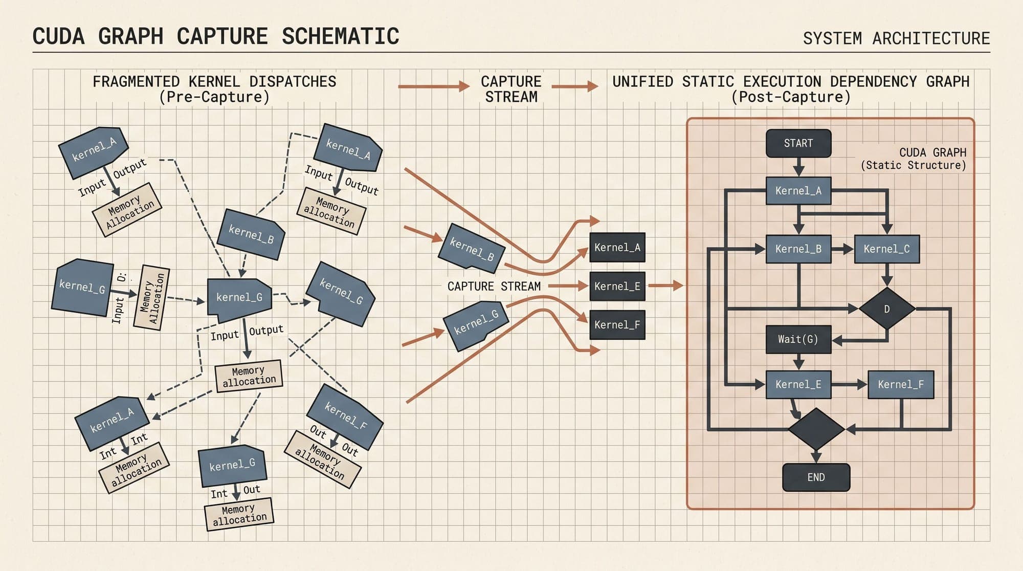
Modern inference engines including vLLM, SGLang, and NVIDIA TensorRT-LLM resolve this bottleneck through CUDA Graph capture. By recording a sequence of discrete CUDA kernel dispatches during engine initialization and instantiating them into an executable graph, runtimes eliminate host-side dispatch overhead. However, adapting static execution graphs to the dynamic workloads of continuous batching, growing sequence lengths, and paged memory structures requires specific architectural strategies: discrete batch bucketing, shared memory pooling, in-place metadata mutation, and piecewise graph compilation.

The CPU Kernel Launch Bottleneck in Autoregressive Decode

During transformer inference, a single forward pass traverses dozens of sequential operations per model layer:

1. Root Mean Square Normalization (RMSNorm) or LayerNorm
2. Query, Key, and Value (QKV) projections
3. Rotary Position Embedding (RoPE) application
4. Attention computation (such as PagedAttention or FlashDecoding)
5. Out-projection GEMMs
6. Gated Multi-Layer Perceptron activations (SwiGLU)
7. Residual tensor additions
8. Distributed communication collectives (NCCL all_reduce or reduce_scatter across Tensor Parallel ranks)

For a 32-layer transformer model running on a single GPU, one decode iteration involves between 250 and 600 discrete kernel launches. On modern server-class hardware like the NVIDIA Hopper H100 or Blackwell B200, each small kernel executes on the GPU in approximately 1 to 5 microseconds. In contrast, standard CPU driver dispatch via the CUDA runtime API incurs an overhead of 2 to 4 microseconds per kernel call due to user-to-kernel space transitions, validation, and queue management.

Standard Eager Execution Stream:
CPU: [ Launch K1 ] -> [ Launch K2 ] -> [ Launch K3 ] -> [ Launch K4 ] ... (High CPU driver overhead)
GPU:      [  K1  ]         [  K2  ]         [  K3  ]         [  K4  ]     (Idle gaps between kernels)

CUDA Graph Execution:
CPU: [ Launch Graph Executable ] (Single driver call, ~5-10 μs)
GPU: [  K1  ][  K2  ][  K3  ][  K4  ] ... (Back-to-back execution without host intervention)

When running eager-mode execution at small batch sizes (such as $B=1$ to $B=16$), the CPU cannot enqueue work fast enough to keep the GPU execution pipeline saturated. The GPU experiences execution bubbles between kernel launches, throttling generation speed to a fraction of available memory bandwidth.

In contrast, the prefill phase processes prompts with hundreds or thousands of tokens simultaneously ($T \gg 1$). The matrix multiplications in prefill execute for tens or hundreds of microseconds per layer, easily masking the CPU dispatch latency. CUDA Graph optimization is therefore primarily critical for the token-by-token decode phase.

CUDA Graph Fundamentals: Capture, Instantiation, and Replay

NVIDIA CUDA Graphs replace stream-based dispatch queues with a defined Directed Acyclic Graph (DAG) of execution nodes.

+-----------------------------------------------------------------------------+
|                         CUDA GRAPH LIFECYCLE                                |
|                                                                             |
|   1. Capture Stream           2. Graph Instantiation    3. Graph Replay     |
|   +-----------------------+   +---------------------+   +---------------+   |
|   | cudaStreamBeginCapture|   | cudaGraphInstantiate|   |cudaGraphLaunch|   |
|   | -> Record Kernel Calls|-->| -> Optimize Node DAG|-->| -> Single API |   |
|   | cudaStreamEndCapture  |   | -> Allocate Handles |   |    Dispatch   |   |
|   +-----------------------+   +---------------------+   +---------------+   |
+-----------------------------------------------------------------------------+

The graph lifecycle consists of three distinct phases:

1. Capture (cudaStreamBeginCapture / cudaStreamEndCapture)

The runtime places a designated CUDA stream into capture mode. Subsequent kernel launches, memory copies, and synchronization events issued to the stream are not executed immediately on hardware; instead, the CUDA driver records the operations and their data dependencies into an in-memory graph representation (cudaGraph_t).

2. Instantiation (cudaGraphInstantiate)

The driver compiles the captured graph into an executable entity (cudaGraphExec_t). During instantiation, the driver analyzes the graph topology, resolves static dependencies, pre-binds GPU execution parameters, and configures hardware work queues. The driver can also perform node fusion and eliminate unnecessary synchronization barriers across independent branches.

3. Replay (cudaGraphLaunch)

At runtime, the host issues a single cudaGraphLaunch call to dispatch the entire pre-compiled sequence. The host runtime overhead drops from several hundred driver interactions to a single invocation taking roughly 5 to 10 microseconds, allowing kernels to execute back-to-back on hardware with zero CPU-induced scheduling bubbles.

The Dynamic Shape Dilemma in LLM Inference

While CUDA Graphs provide substantial execution efficiency, they impose strict invariants defined by the underlying GPU hardware runtime:

• Fixed Tensor Memory Addresses: Kernel argument structures store explicit physical 64-bit GPU virtual memory pointers. Memory addresses cannot be reallocated or remapped between graph replays without graph destruction.
• Fixed Grid and Block Dimensions: Execution geometry (thread block count and thread count per block) is compiled statically into each graph node.
• Fixed Intermediate Buffer Shapes: Tensor dimensions allocated during graph capture must remain constant during subsequent executions.

These constraints conflict directly with the dynamic operational characteristics of production LLM serving:

1. Continuous (In-Flight) Batching: The active request count fluctuates continuously as individual sequences finish and new requests enter the decode pool.
2. Variable Sequence Lengths: Every generation step increments the context length of active sequences by one token, requiring dynamic key-value cache lookups.
3. Paged Memory Indirection: Runtimes like vLLM allocate non-contiguous KV cache blocks in physical GPU memory via PagedAttention, where virtual-to-physical block tables change on every scheduling step.

Serving engines resolve this conflict by structuring execution around four complementary architectural patterns.

Architectural Solutions in Production Runtimes

1. Discrete Batch Size Bucketing and Dummy Padding

Because capturing a separate graph for every possible integer batch size from 1 to 512 is prohibitively expensive in terms of initialization latency and host memory, engines employ discrete batch size bucketing.

At startup, the engine selects a curated set of batch sizes (for example, $B \in \{1, 2, 4, 8, 16, 24, 32, 48, 64, 96, 128, 160, 192, 224, 256\}$). The engine captures and instantiates one dedicated CUDA graph for each bucket.

# Conceptual batch bucketing logic in serving runtime
CAPTURED_BUCKETS = [1, 2, 4, 8, 16, 24, 32, 48, 64, 96, 128, 192, 256]

def select_graph_bucket(active_batch_size: int) -> int:
    for bucket in CAPTURED_BUCKETS:
        if bucket >= active_batch_size:
            return bucket
    raise RuntimeError(f"Batch size {active_batch_size} exceeds max bucket")

When the iteration scheduler forms a decode batch containing $N$ requests:

1. The engine identifies the smallest pre-captured bucket $B_{\text{bucket}} \ge N$.
2. The engine populates the first $N$ slots of the static input tensor with active request tokens and metadata.
3. The remaining $B_{\text{bucket}} - N$ slots are filled with dummy padding tokens (typically token ID 0 pointing to a dedicated scratch memory block).
4. The corresponding CUDA graph for $B_{\text{bucket}}$ is launched.
5. The engine extracts the first $N$ generated logits or sampled tokens, discarding the padding positions.

2. Static Memory Pooling (graph_pool_handle)

If every batch-bucket graph independently allocated its own intermediate layer activation buffers, GPU VRAM consumption would scale linearly with the number of buckets, starving the KV cache pool.

Modern frameworks leverage PyTorch's native CUDA Graph memory pool integration (torch.cuda.graph_pool_handle() or torch.cuda.CUDAGraph(pool=...)) and CUDA's memory pool APIs (cudaMemPool_t). Runtimes capture graphs in descending order of batch size (from $B=256$ down to $B=1$). The largest batch size graph establishes the memory arena high-water mark; smaller graphs reuse the existing static activation buffers within that shared pool, ensuring zero additional VRAM consumption across bucket variations.

import torch

# Share a single global graph pool across all batch buckets
graph_pool = torch.cuda.graph_pool_handle()

captured_graphs = {}
for batch_size in sorted(CAPTURED_BUCKETS, reverse=True):
    graph = torch.cuda.CUDAGraph()
    
    # Run warmup execution before capture
    model.forward_decode(static_inputs[batch_size])
    torch.cuda.synchronize()
    
    # Capture using shared memory pool
    with torch.cuda.graph(graph, pool=graph_pool):
        static_outputs[batch_size] = model.forward_decode(static_inputs[batch_size])
    
    captured_graphs[batch_size] = graph

3. In-Place Input Buffer and Pointer Mutation

To run static graphs with dynamic request states, engines pre-allocate static device tensors for all model inputs:

• static_input_ids: Tensor of shape [max_batch_size]
• static_positions: Tensor of shape [max_batch_size]
• static_block_tables: PagedAttention block mapping tensor of shape [max_batch_size, max_blocks_per_seq]
• static_slot_mapping: Direct memory slot offsets of shape [max_batch_size]

Prior to calling graph.replay(), the host scheduler copies the dynamic metadata for the active batch into the static input buffers via an asynchronous host-to-device memory copy (cudaMemcpyAsync) on the main stream. Because the GPU virtual memory address of the static tensor never changes, the pre-recorded kernels read the updated request state and write KV cache states into the appropriate physical memory blocks without invalidating the graph topology.

4. Piecewise CUDA Graphs and Dynamic Exits

Certain operations cannot be safely captured inside a monolithic CUDA graph:

• Dynamic tensor-parallel collectives that adapt across varying node topologies
• Memory-bound fallback kernels for extreme sequence lengths
• Cascade attention mechanisms and multi-tier speculative verifications

Runtimes utilize piecewise CUDA graph compilation (as documented in vLLM's torch.compile architecture). The compiler decomposes the model computation graph into graph-safe linear subgraphs separated by dynamic boundary nodes. Safe segments run as compiled CUDA graphs, while dynamic operations execute as compiled Triton kernels or eager operations.

Multi-Step Scheduling and Speculative Verification

In standard serving architectures, the engine executes a CPU scheduling cycle between every generated token. Even with CUDA Graphs eliminating kernel launch latency, the CPU scheduler still consumes 100 to 300 microseconds per iteration evaluating priority queues, updating token histories, and checking stop criteria.

Single-Step Scheduling:
[ CPU Schedule ] -> [ CUDA Graph (1 Step) ] -> [ CPU Schedule ] -> [ CUDA Graph (1 Step) ]
(Host-device round-trip latency incurred on every generated token)

Multi-Step Scheduling (K=4):
[ CPU Schedule ] -> [ CUDA Graph Replay Loop: 4 Decode Steps on GPU ] -> [ CPU Verification ]
(CPU scheduler runs once every K tokens, amortizing host overhead across multiple steps)

To break this host scheduling ceiling, runtimes deploy Multi-Step Scheduling. The serving engine instructs the GPU to execute a fixed sequence of $K$ decode iterations (typically $K \in [4, 16]$) autonomously. The CUDA graph encapsulates the decode forward pass, sampling kernel, and in-place input feedback loop directly on device:

1. Token $t$ is generated and sampled on the GPU.
2. An on-device update kernel writes token $t$ directly into the static input buffer for step $t+1$.
3. The graph executes the subsequent step without synchronizing with the host CPU.
4. The host checks completion status only once every $K$ steps.

In speculative decoding pipelines, CUDA Graphs accelerate both the draft model rollouts and target model verification passes. The draft model runs multi-step graph loops to generate speculative candidate trees, which are verified in a single batch-padded target model graph execution.

Operational Trade-Offs and Best Practices

Deploying CUDA Graphs in enterprise production environments requires balancing memory constraints, startup latency, and inference throughput:

Production Configuration Profiles

• Default Profile: Powers-of-two batch bucketing up to 128. Requires 15 to 30 seconds warmup latency with baseline memory pool allocation. Yields 1.5 to 2.5 ms kernel launch savings per decode step.
• Aggressive Latency Profile: Dense batch buckets (1, 2, 4, 8, 12, 16, 24, 32, 48, 64). Requires 45 to 90 seconds warmup latency with a 5% scratch margin. Yields up to 3.0 ms launch savings per step.
• High-Concurrency Throughput Profile: Extended batch buckets up to 256 or 512. Requires 60 to 120 seconds warmup latency with a 15% high-water buffer. Yields 2.0 to 4.0 ms launch savings per step.

Production Implementation Guidelines

• Order of Capture: Always capture graphs from largest batch size to smallest. This guarantees that PyTorch and CUDA allocate the maximum required workspace upfront, avoiding secondary memory allocations during lower batch captures.
• Warmup Iterations: Perform at least one full eager forward pass on dummy inputs before calling cudaStreamBeginCapture. This initializes internal runtime state, driver context tables, and framework caches that might otherwise trigger un-capturable allocation calls.
• NCCL Collective Alignment: When using Tensor Parallelism ($TP > 1$), ensure all participating ranks initiate and complete graph capture synchronously. Inter-GPU communicators must use pre-allocated static communication buffers to prevent collective deadlocks during graph replay.
• Nsight Systems Profiling: Profile the inference engine using NVIDIA Nsight Systems (nsys profile --trace=cuda,nvtx,osrt). A properly tuned CUDA Graph deployment exhibits continuous GPU kernel execution timelines with zero white space or CPU dispatch gaps between attention and MLP blocks.

Sources

• vLLM CUDA Graphs Architecture and Compilation Design
• SGLang CUDA Graph Optimization and Decode Acceleration
• NVIDIA CUDA C++ Programming Guide: CUDA Graphs
• PyTorch CUDA Graphs Documentation and Memory Pooling (torch.cuda.CUDAGraph)
• vLLM Architecture: Introduction to torch.compile and CUDA Graphs Integration
• NVIDIA TensorRT-LLM Architecture and Performance Optimization Guide