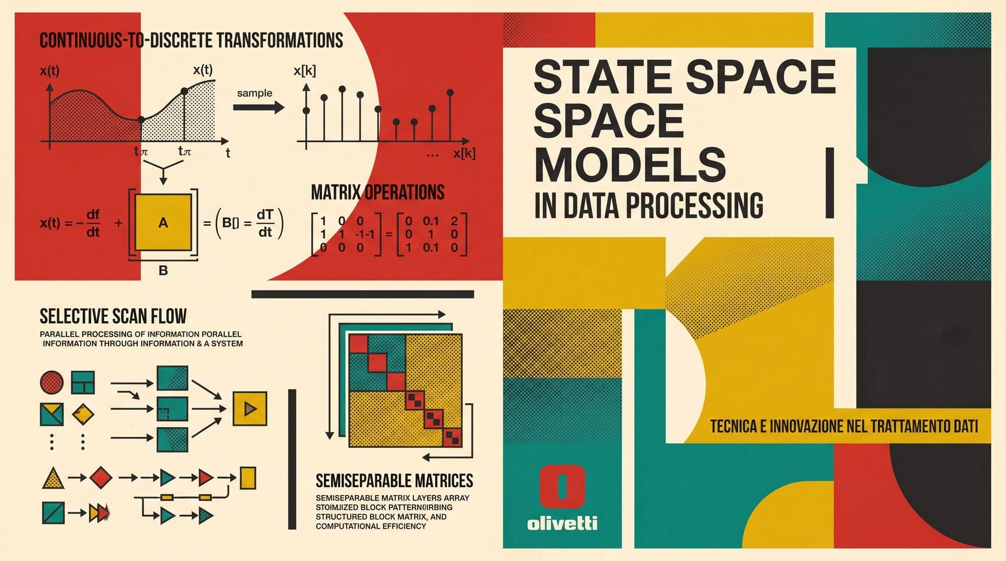
State Space Models (SSMs) and Mamba: Mathematical Foundations of Continuous-Time Discretization, Selective Scan Mechanics, and Structured State Space Duality

Autoregressive Large Language Models (LLMs) built on the standard Transformer architecture rely on softmax self-attention. While self-attention provides expressive in-context learning and dense token-to-token associative recall, it exhibits fundamental algorithmic scaling limits: prefill compute scales quadratically with sequence length ($O(L^2 d)$), and autoregressive token generation requires maintaining a Key-Value (KV) cache that grows linearly with sequence length ($O(L d)$). At context windows spanning hundreds of thousands of tokens, the KV cache saturates GPU High-Bandwidth Memory (HBM), converting inference into a memory-bandwidth-bound workload.

State Space Models (SSMs) offer an alternative mathematical formulation for sequence modeling. Rooted in continuous-time control theory, modern deep SSMs achieve linear-time computation ($O(L d)$) during training and constant-state memory footprint ($O(1)$ per step) during autoregressive decoding. This explainer covers the mathematical evolution of deep state space architectures: from continuous-time linear time-invariant (LTI) differential equations and HiPPO memory matrices, to discrete convolutions, the input-dependent selective scan mechanism of Mamba (S6), and the unified matrix formulation of Structured State Space Duality (SSD) in Mamba-2.

1. The Mathematical Origin: Continuous-Time Linear Time-Invariant Systems

A continuous-time State Space Model maps a 1-dimensional input signal $x(t) \in \mathbb{R}$ to a 1-dimensional output signal $y(t) \in \mathbb{R}$ through an $N$-dimensional latent state variable $h(t) \in \mathbb{R}^N$. The continuous system is governed by a pair of linear differential equations:

$$\dot{h}(t) = A h(t) + B x(t)$$

$$y(t) = C h(t) + D x(t)$$

Here:

• $A \in \mathbb{R}^{N \times N}$ is the state transition matrix, determining how the latent state evolves independently of inputs.
• $B \in \mathbb{R}^{N \times 1}$ is the input projection matrix, mapping the scalar input into the state vector.
• $C \in \mathbb{R}^{1 \times N}$ is the output projection matrix, mapping the latent state back to the output domain.
• $D \in \mathbb{R}^{1 \times 1}$ is a direct feedthrough skip connection (often treated as $D x_t$ with a learned scalar parameter or omitted for clarity).

For multi-dimensional hidden feature channels $D_{\text{in}}$, the system is typically applied independently across each feature dimension using broadcasted or diagonalized parameters.

                  +---------+
    x(t) -------->|    B    |--------(+)-------------> h'(t) ---> [ \int dt ] ---> h(t) ---+---> C ---> (+) ---> y(t)
      |           +---------+          ^                                                |         ^
      |                                |                      +---------+               |         |
      |                                +----------------------|    A    |<--------------+         |
      |                                                       +---------+                         |
      +------------------------------------------------------ D ----------------------------------+

The HiPPO Framework and Memory Initialization

If matrix $A$ is randomly initialized, the state $h(t)$ rapidly suffers from either exponential vanishing or exploding gradients over long temporal sequences. To address this, the HiPPO (High-order Polynomial Projection Operators) framework constructs the state transition matrix $A$ to maintain an optimal online polynomial approximation of the continuous input history $x_{\le t}$ with respect to a defined probability measure.

Under the continuous scaled Legendre polynomial measure (HiPPO-LegS), the transition matrix $A \in \mathbb{R}^{N \times N}$ and input matrix $B \in \mathbb{R}^{N \times 1}$ are defined analytically:

$$A_{nk} = -\begin{cases} \sqrt{2n+1}\sqrt{2k+1} & \text{if } n > k \\ n+1 & \text{if } n = k \\ 0 & \text{if } n < k \end{cases}$$

$$B_n = \sqrt{2n+1}$$

for $n, k \in \{0, 1, \dots, N-1\}$. The diagonal entries $A_{nn} = -(n+1)$ ensure that all eigenvalues have strictly negative real components ($\text{Re}(\lambda) < 0$), guaranteeing that the differential equation remains exponentially stable over continuous time intervals.

2. Discretization Transforms: Bridging Continuous Systems to Discrete Data

Digital sequence models process discrete token sequences $(x_0, x_1, \dots, x_{L-1})$ rather than continuous functions $x(t)$. Discretization converts the continuous parameters $(A, B, C)$ into discrete recurrence matrices $(\bar{A}, \bar{B}, \bar{C})$ parameterized by a continuous positive step-size parameter $\Delta > 0$.

Zero-Order Hold (ZOH) Discretization

The standard discretization method used in deep SSMs is the Zero-Order Hold (ZOH) transform. ZOH assumes that the input signal remains constant over the discrete interval $[t \Delta, (t+1)\Delta)$:

$$x(\tau) = x_t \quad \text{for } \tau \in [t \Delta, (t+1)\Delta)$$

Integrating the continuous state equation over the interval yields the exact analytical solution:

$$h_t = h(t\Delta) = \exp(\Delta A) h_{t-1} + \left( \int_0^\Delta \exp(s A) \, ds \right) B x_t$$

Evaluating the matrix integral produces the discrete recurrence parameters:

$$\bar{A} = \exp(\Delta A)$$

$$\bar{B} = (\Delta A)^{-1} (\exp(\Delta A) - I) \cdot \Delta B$$

$$\bar{C} = C$$

When computed numerically or under first-order Taylor expansions for small $\Delta$, the input parameter simplifies to $\bar{B} \approx \Delta B$.

Bilinear (Tustin) Transform

An alternative discretization approach is the Bilinear (Tustin) transform, which applies a trapezoidal integration approximation:

$$\bar{A} = \left( I - \frac{\Delta}{2} A \right)^{-1} \left( I + \frac{\Delta}{2} A \right)$$

$$\bar{B} = \left( I - \frac{\Delta}{2} A \right)^{-1} \Delta B$$

The ZOH formulation preserves the continuous-time system dynamics across variable step sizes $\Delta$, giving the model resolution-invariance and providing a principled mathematical mechanism for continuous-time interpolation.

3. The Dual Representation: Linear Recurrence and Fast Convolution

When the parameters $(\bar{A}, \bar{B}, \bar{C})$ are invariant over time (Linear Time-Invariant, or LTI), the system possesses a dual mathematical representation: a step-by-step recurrence and an explicit global 1D convolution.

Recurrent Representation (Linear-Time Generation)

Unrolling the discretized state equation yields a first-order vector recurrence:

$$h_t = \bar{A} h_{t-1} + \bar{B} x_t$$

$$y_t = \bar{C} h_t$$

During autoregressive generation, computing output $y_t$ given $x_t$ requires only multiplying the state vector $h_{t-1} \in \mathbb{R}^N$ by $\bar{A}$, adding $\bar{B} x_t$, and projecting through $\bar{C}$. This operation requires $O(1)$ memory state and $O(N)$ arithmetic operations per token, completely avoiding the need to cache prior key-value activations.

Step t-1:  h_{t-1} ------(\times \bar{A})-----> (+) ------> h_t ------> (\times \bar{C}) ------> y_t
                                                 ^
                                                 |
Step t:    x_t ----------(\times \bar{B})--------+

Convolutional Representation (Parallel Training)

Assuming initial state $h_{-1} = 0$, expanding the recurrence over an entire sequence of length $L$ reveals an explicit convolutional structure:

$$h_0 = \bar{B} x_0$$

$$h_1 = \bar{A} \bar{B} x_0 + \bar{B} x_1$$

$$h_2 = \bar{A}^2 \bar{B} x_0 + \bar{A} \bar{B} x_1 + \bar{B} x_2$$

$$y_t = \bar{C} h_t = \sum_{j=0}^t \bar{C} \bar{A}^{t-j} \bar{B} x_j$$

This summation is an exact discrete 1D convolution between the input sequence $x \in \mathbb{R}^L$ and an explicit SSM convolution filter $\bar{K} \in \mathbb{R}^L$:

$$y = x * \bar{K}$$

$$\bar{K} = \left( \bar{C}\bar{B}, \; \bar{C}\bar{A}\bar{B}, \; \bar{C}\bar{A}^2\bar{B}, \; \dots, \; \bar{C}\bar{A}^{L-1}\bar{B} \right)$$

In early deep SSM architectures such as S4 (Structured State Spaces) and H3 (Hungry Hungry Hippos), the filter $\bar{K}$ was computed efficiently using diagonal plus low-rank Cauchy kernels. Once computed, the full output sequence $y$ was calculated in parallel across all $L$ tokens via Fast Fourier Transforms (FFT):

$$y = \mathcal{F}^{-1} \left( \mathcal{F}(x) \odot \mathcal{F}(\bar{K}) \right)$$

This reduced parallel training time complexity to $O(L \log L)$.

   Training Mode:   Parallel FFT Convolution  -->  O(L \log L) compute, highly parallel
   Inference Mode:  Recurrent State Update    -->  O(1) memory state, O(1) time per token

4. The Selectivity Bottleneck: Why LTI Models Fail at Language

Despite the theoretical efficiency of LTI models, empirical evaluations showed they lagged behind Transformers on language modeling benchmarks. The core limitation lies in the mathematical definition of Time-Invariance.

In an LTI model, the convolution kernel $\bar{K}$ is static and completely independent of the input tokens $x$. The weights assigned to token $x_{t-k}$ depend solely on relative distance $k$, not on the semantic content of $x_{t-k}$ or the current context.

LTI SSM:    Memory decay is static across time.
            Noise tokens receive the exact same state updates as critical keywords.

Selective:  Memory decay is input-dependent.
            The model resets state upon encountering irrelevant tokens, and stores critical facts indefinitely.

An LTI system cannot perform two essential foundational tasks required for language understanding:

1. Selective Copying: Memorizing specific informational tokens from a noisy prompt while zeroing out irrelevant filler tokens.
2. Induction Heads (Associative Recall): Detecting a pattern [A] [B] ... [A] and dynamically retrieving token [B] based on content similarity.

5. Mamba (S6): Input-Dependent Selective State Spaces

To overcome the expressivity barrier of LTI models, Mamba introduced the Selective State Space mechanism (referred to in the literature as S6). Mamba makes the discretization parameters dynamic functions of the input token at each timestep:

$$B_t = \text{Linear}_N(x_t) \in \mathbb{R}^{B \times L \times N}$$

$$C_t = \text{Linear}_N(x_t) \in \mathbb{R}^{B \times L \times N}$$

$$\Delta_t = \text{Softplus}\left( \text{Parameter}_\Delta + \text{Linear}_D(x_t) \right) \in \mathbb{R}^{B \times L \times D}$$

$$\bar{A}_t = \exp(\Delta_t A), \quad \bar{B}_t = \Delta_t B_t$$

Because $\bar{A}_t$ and $\bar{B}_t$ now vary at every timestep $t$, the system becomes a Linear Time-Varying (LTV) system.

                           +-------------------------------------+
                           |            Input Token x_t          |
                           +-------------------------------------+
                             |                 |               |
                             v                 v               v
                        Linear_D(x_t)    Linear_N(x_t)   Linear_N(x_t)
                             |                 |               |
                             v                 v               v
                         Step Size \Delta_t    Input B_t       Output C_t
                             |                 |               |
                             +--------+--------+               |
                                      |                        |
                                      v                        |
               h_t = exp(\Delta_t A) h_{t-1} + (\Delta_t B_t) x_t     |
                                      |                        |
                                      v                        |
                                    y_t = C_t h_t <------------+

Mechanics of the Selection Mechanism

The input-dependent step size $\Delta_t$ acts as a generalized gating mechanism:

• Large $\Delta_t$: Causes $\bar{A}_t \to 0$ (decaying prior historical state) while amplifying $\bar{B}_t \to \Delta_t B_t$ (writing current token $x_t$ into state $h_t$).
• Small $\Delta_t$: Causes $\bar{A}_t \to I$ (preserving long-term historical state) while ignoring current input ($\bar{B}_t \to 0$).

Hardware-Aware Parallel Associative Scan

Because the system is time-varying, it can no longer be computed via static FFT convolutions. A sequential loop would require $O(L)$ sequential memory round-trips to GPU High-Bandwidth Memory (HBM), causing severe memory-bandwidth starvation.

To achieve parallel training, Mamba formulates the recurrence as a Parallel Associative Scan. The state recurrence $h_t = \bar{A}_t h_{t-1} + \bar{B}_t x_t$ is transformed into a prefix product under a binary associative operator $\circ$:

$$(a_2, b_2) \circ (a_1, b_1) = (a_2 a_1, \; a_2 b_1 + b_2)$$

where $a_t = \bar{A}_t$ and $b_t = \bar{B}_t x_t$.

Associativity Verification:
  [(a_3, b_3) \circ (a_2, b_2)] \circ (a_1, b_1)
    = (a_3 a_2, a_3 b_2 + b_3) \circ (a_1, b_1)
    = (a_3 a_2 a_1, (a_3 a_2) b_1 + (a_3 b_2 + b_3))
    = (a_3 a_2 a_1, a_3 a_2 b_1 + a_3 b_2 + b_3)

  (a_3, b_3) \circ [(a_2, b_2) \circ (a_1, b_1)]
    = (a_3, b_3) \circ (a_2 a_1, a_2 b_1 + b_2)
    = (a_3 (a_2 a_1), a_3 (a_2 b_1 + b_2) + b_3)
    = (a_3 a_2 a_1, a_3 a_2 b_1 + a_3 b_2 + b_3)

Because the operator $\circ$ is strictly associative, the sequence of cumulative states $(h_0, h_1, \dots, h_{L-1})$ is evaluated in parallel in $O(\log L)$ parallel steps using a Blelloch parallel prefix scan tree on GPU SRAM:

Step 0:   (a_0, b_0)      (a_1, b_1)      (a_2, b_2)      (a_3, b_3)
              \              /                \              /
               \            /                  \            /
Step 1:         (a_{01}, b_{01})                (a_{23}, b_{23})
                       \                               /
                        \                             /
Step 2:                        (a_{0123}, b_{0123})

The Mamba kernel fuses the computation directly inside GPU SRAM: parameters $\Delta_t, B_t, C_t$ are loaded from HBM into fast on-chip SRAM, discretized, scanned, multiplied by $C_t$, and written back to HBM once, avoiding intermediate memory materialization.

6. Mamba-2 and Structured State Space Duality (SSD)

While Mamba achieved linear-time scaling and matched Transformer performance, the associative scan algorithm runs primarily on standard GPU arithmetic logic units (ALUs), which deliver substantially lower theoretical TFLOPs than Tensor Cores designed for dense Matrix Multiply-Accumulate (MMA) operations.

In Mamba-2, Dao and Gu established Structured State Space Duality (SSD): a formal mathematical proof showing that Selective State Space Models and Masked Linear Attention are equivalent dual representations of 1-semiseparable matrix transformations.

                 +---------------------------------------------+
                 |       Structured State Space Duality        |
                 +---------------------------------------------+
                                /               \
                               /                 \
                              v                   v
                   Selective SSMs             Linear Attention
                (State-Space Recurrence)    (Matrix Multiplication)
                              \                   /
                               \                 /
                                v               v
                    +---------------------------------------+
                    |  1-Semiseparable Matrix Computation   |
                    |    Fused Chunkwise Tensor Core GEMMs  |
                    +---------------------------------------+

The Semiseparable Matrix Equivalence

Consider the global transformation mapping an input sequence $X \in \mathbb{R}^{L \times D}$ to an output sequence $Y \in \mathbb{R}^{L \times D}$. The entire transformation can be written as a single lower-triangular matrix multiplication:

$$Y = M X$$

where matrix $M \in \mathbb{R}^{L \times L}$ has entries:

$$M_{j, i} = \begin{cases} C_j^\top \left( \prod_{k=i+1}^j \bar{A}_k \right) \bar{B}_i & \text{if } j > i \\ C_i^\top \bar{B}_i & \text{if } j = i \\ 0 & \text{if } j < i \end{cases}$$

When $\bar{A}_t = \alpha_t I$ is constrained to a scalar-times-identity matrix per attention head (where $\alpha_t = \exp(\Delta_t a)$ for a learned scalar $a \le 0$), the transformation factorizes cleanly into a masked attention kernel:

$$M = \left( C B^\top \right) \odot G$$

where $G_{j, i} = \prod_{k=i+1}^j \alpha_k$ is a scalar decay matrix. Defining $Q = C$, $K = B$, and $V = X$, the output becomes:

$$Y = \left( (Q K^\top) \odot G \right) V$$

This formulation reveals that Mamba is mathematically equivalent to a causal Linear Attention mechanism with an explicit data-controlled exponential decay mask $G$.

The Chunkwise SSD Algorithm

To exploit Tensor Cores on NVIDIA Hopper and Blackwell architectures, Mamba-2 replaces the fine-grained token-level associative scan with a Chunkwise Decomposition:

1. Partitioning: The sequence of length $L$ is split into contiguous chunks of length $Q$ (typically $Q = 64$ or $128$).
2. Intra-Chunk Computation (Local Attention): Within each chunk, tokens interact directly via dense matrix multiplication:

$$Y_{\text{local}}^{(k)} = \left( (Q^{(k)} (K^{(k)})^\top) \odot G^{(k)} \right) V^{(k)}$$ This is executed as a dense GEMM using Tensor Cores in $O(Q^2)$ arithmetic operations per chunk.

1. Inter-Chunk State Passing (Global Recurrence): Each chunk summarizes its historical context into an exit state $H^{(k)} \in \mathbb{R}^{N \times P}$:

$$H^{(k)} = \alpha^{(k)} H^{(k-1)} + (K^{(k)})^\top V^{(k)}$$

1. Output Reconstruction: The inter-chunk state is projected into the current chunk via $Q^{(k)} H^{(k-1)}$ and added to $Y_{\text{local}}^{(k)}$.

Chunk k-1:  [ Token 0 ... Token 63 ]  --->  Exit State H^{(k-1)}
                                                        |
                                                        v (\times \alpha^{(k)})
Chunk k:    [ Token 64 ... Token 127 ] --->  Intra-Chunk GEMM  +  (Q^{(k)} \times H^{(k-1)}) ---> Y^{(k)}
                                                        |
                                                        v
                                             Exit State H^{(k)}

By decomposing the computation into intra-chunk matrix multiplications and inter-chunk state updates, the Chunkwise SSD algorithm runs at over $85\%$ of peak Tensor Core utilization, achieving $2\times$ to $8\times$ training throughput speedups over Mamba-1.

7. Mathematical and Algorithmic Comparison

The architectural trade-offs between standard Softmax Attention, Linear Attention, Mamba-1 (S6), and Mamba-2 (SSD) can be summarized across their computational dimensions:

| Dimension | Softmax Attention (Transformer) | Standard Linear Attention | Mamba-1 (S6) | Mamba-2 (SSD) | | :--- | :--- | :--- | :--- | :--- | | Prefill Compute Complexity | $O(L^2 d)$ | $O(L d^2)$ | $O(L d N)$ | $O(L d N)$ (Tensor Core GEMM) | | Generation Memory (Per Step) | $O(L d)$ (Linear KV Cache) | $O(d^2)$ (Constant State) | $O(d N)$ (Constant State) | $O(d N)$ (Constant State) | | Decay / Gating Mechanism | Dynamic Softmax Sim. | Static / None | Input-dependent $\Delta_t A$ | Input-dependent $\Delta_t A$ (Scalar-Identity) | | Primary Compute Primitive | FlashAttention GEMM | Sequential / Scan | Associative Scan (ALU bound) | Chunked GEMM (Tensor Core bound) | | Associative Recall (In-Context) | Exact / Full Capacity | Low / Degraded | High | High | | State Parameter Rank | Full Rank ($L$) | Low Rank ($d$) | Low Rank ($N$) | Head Rank ($N$) |

8. Hybrid Architectures and Production Serving Economics

While pure SSM models exhibit linear prefill scaling and constant decoding memory, Transformer self-attention retains an inherent advantage in precise associative lookup across massive, unstructured context windows (e.g. retrieving arbitrary key-value hashes from 100K+ token documents).

To capture the benefits of both paradigms, production systems have adopted Hybrid SSM-Transformer Architectures:

• Jamba (AI21 Labs): Interleaves Mamba layers with Transformer attention layers and Mixture of Experts (MoE) feedforward blocks in a structured $1:7$ or $1:3$ ratio (e.g., 1 attention layer for every 7 Mamba layers).
• Nemotron-4 / Bamba (NVIDIA): Combines Mamba-2 SSD layers with periodic full-attention blocks, reducing KV cache memory consumption by $80\text{--}90\%$ while matching pure Transformer accuracy on long-context retrieval benchmarks.

Hybrid Pipeline Block:
  [ Mamba-2 Layer ] -> [ Mamba-2 Layer ] -> [ Mamba-2 Layer ] -> [ Attention Layer (KV Cache) ]
  \_____________________________________ ____________________________________/
                                        v
                       Saves ~75-85% KV Cache Memory Footprint

Production Serving Economics

In high-concurrency LLM serving environments, GPU memory capacity is dominated by the KV cache. By reducing the number of attention layers from $N_{\text{layers}}$ to $N_{\text{layers}} / 8$:

1. Serving Memory Footprint: The memory required per concurrent user drops from gigabytes to tens of megabytes, allowing serving engines to increase maximum batch sizes by $4\times$ to $10\times$.
2. Throughput Scaling: Serving engines become compute-bound rather than memory-bandwidth-bound during generation, significantly reducing cost per million generated tokens.

Sources

• Gu, A., & Dao, T. (2023). Mamba: Linear-Time Sequence Modeling with Selective State Spaces. arXiv:2312.00752.
• Dao, T., & Gu, A. (2024). Transformers are SSMs: Generalized Models and Efficient Algorithms Through Structured State Space Duality. arXiv:2405.21060.
• Gu, A., Dao, T., Dao, S., Goel, K., Dao, A., Rudra, A., & Ré, C. (2020). HiPPO: Recurrent Memory with Optimal Polynomial Projections. arXiv:2008.07669.
• Gu, A., Goel, K., & Ré, C. (2021). Efficiently Modeling Long Sequences with Structured State Spaces. arXiv:2111.00396.
• Fu, D. Y., Dao, T., Saab, K. K., Thomas, A. W., Rudra, A., & Ré, C. (2022). Hungry Hungry Hippos: Towards Language Modeling with State Space Models. arXiv:2212.14052.
• AI21 Labs. (2024). Jamba: A Hybrid Transformer-Mamba Language Model. arXiv:2403.19887.
• Katharopoulos, A., Vyas, A., Pappas, N., & Fleuret, F. (2020). Transformers are RNNs: Fast Autoregressive Transformers with Linear Attention. arXiv:2006.16236.