Neural Tangent Kernel: How Infinite-Width Networks Linearize Gradient Descent

title: "Neural Tangent Kernel: How Infinite-Width Networks Linearize Gradient Descent" slug: "neural-tangent-kernel-how-infinite-width-networks-linearize-gradient-descent" feature_image: "https://cms.llms.blog/content/images/2026/08/neural-tangent-kernel-cover.png" tags: ["edu", "theory", "foundations"] status: published

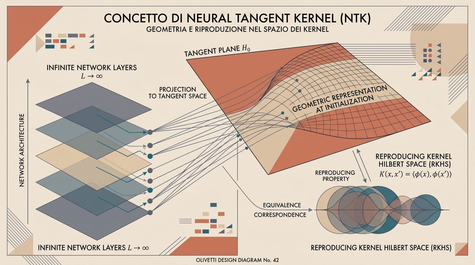
The Neural Tangent Kernel (NTK) describes the behavior of infinitely wide neural networks during gradient descent. In the infinite-width limit, network training reduces to kernel regression with a fixed kernel — the NTK — that stays constant throughout training. This theoretical framework explains why wide networks converge to global minima, why they struggle to learn high-frequency functions early (spectral bias), and why they behave differently from finite-width networks that learn features.

From Finite to Infinite Width

A finite neural network with parameters $\theta$ computes a function $f(x; \theta)$ . Under gradient flow on loss $\mathcal{L} = \frac{1}{2}\sum_i (f(x_i; \theta) - y_i)^2$ , the output evolves as:

$\frac{d f(x; \theta_t)}{dt} = \sum_i \Theta_t(x, x_i) (y_i - f(x_i; \theta_t))$

where $\Theta_t(x, x') = \nabla_\theta f(x; \theta_t)^\top \nabla_\theta f(x'; \theta_t)$ is the empirical NTK at time $t$ .

Jacot, Gabriel, and Hongler (2018) showed that as width $n \to \infty$ , two things happen simultaneously [^1]:

Initialization convergence: $\Theta_0(x, x') \to \Theta_\infty(x, x')$ deterministically.
Training constancy: $\Theta_t(x, x') \to \Theta_\infty(x, x')$ for all $t \ge 0$ .

The network output then follows a linear ODE with a fixed kernel, solvable in closed form:

$f_t(x) = f_0(x) + \Theta_\infty(x, X) \Theta_\infty(X, X)^{-1} (I - e^{-t \Theta_\infty(X, X)}) (y - f_0(X))$

At $t \to \infty$ , this converges to the kernel ridgeless regression solution — the minimum-norm interpolant in the RKHS of $\Theta_\infty$ .

Lazy Training vs Feature Learning

The NTK regime is often called lazy training because parameters barely move from initialization: $\|\theta_t - \theta_0\| \sim O(1/\sqrt{n})$ . The network operates as a linear model over fixed random features $\phi(x) = \nabla_\theta f(x; \theta_0)$ .

This contrasts with feature learning in finite-width networks, where hidden representations adapt to the task. In the NTK limit, the representation is frozen at initialization — the network cannot discover new features, only recombine the initial random projection.

Practical consequence: If you scale learning rate as $\eta \propto 1/n$ (standard parametrization), you enter the NTK regime. The network fits a kernel model but fails to learn hierarchical features. This is why standard parametrization requires careful width scaling to maintain feature learning [^2].

Spectral Bias and Frequency Learning

The NTK's eigen-decomposition on the data distribution reveals spectral bias: the kernel's eigenfunctions correspond to functions of different frequencies, with eigenvalues decaying for higher frequencies. Training fits low-frequency components first; high-frequency components require exponentially more time [^3].

This matches empirical observations:

Wide networks learn low-frequency patterns quickly but struggle with sharp boundaries and fine details early in training.
The NTK of ReLU networks has polynomial eigenvalue decay, so high-frequency learning is slow but not impossible.
Architectural choices (depth, activation, normalization) reshape the NTK spectrum.

NTK and Architecture Design

Depth and Residual Connections

Deeper networks in the NTK limit can suffer from kernel depth degradation: the NTK becomes degenerate, losing expressivity. Residual connections (ResNet) preserve the NTK's conditioning by maintaining signal propagation — the skip connections keep the kernel well-behaved as depth increases [^4].

Normalization

Batch normalization and layer normalization break NTK constancy. They introduce data-dependent scaling that evolves during training, pushing the network out of the lazy regime and enabling feature learning even at large width [^5].

Attention and Transformers

The NTK of attention mechanisms has been characterized: self-attention at initialization yields a kernel that depends on token positions and values. However, transformer NTKs exhibit different spectral properties than MLPs, with implications for long-context extrapolation [^6].

Maximal Update Parametrization (μP)

The NTK limitation — frozen features — led to μP (Maximal Update Parametrization) [^7]. By scaling initialization and learning rates differently (weights $\sim 1/\sqrt{n}$ , learning rate constant, output scaled by $1/n$ ), μP enables feature learning in the infinite-width limit. The network no longer linearizes; hidden representations evolve, and the limiting object is a tensor program rather than a fixed kernel.

μP is now standard for large language model pre-training (GPT-3, PaLM, LLaMA families use μP-compatible scaling). It allows hyperparameter transfer: optimal learning rates found on small μP models transfer directly to large ones.

NTK-Aware Positional Encoding (RoPE Scaling)

The NTK's spectral bias insight was applied to rotary position embeddings (RoPE). Standard RoPE interpolation stretches all frequencies uniformly, degrading high-frequency precision. NTK-Aware RoPE scaling (bloc97, 2023) applies non-linear frequency scaling derived from NTK theory: low frequencies interpolate more aggressively, high frequencies are preserved [^8]. This formed the basis for YaRN and LongRoPE context extension methods.

Limitations of the NTK Framework

| Aspect | NTK Prediction | Reality in Finite Networks | |--------|----------------|----------------------------| | Feature learning | None (frozen at init) | Core to deep learning success | | Generalization | Kernel RKHS norm | Implicit regularization, flat minima | | Scaling laws | Power-law with width | More complex, includes feature learning | | Transfer learning | Kernel alignment | Representation adaptation |

The NTK is a first-order approximation valid only in the infinite-width limit with standard parametrization. It does not capture:

Representation learning and hierarchical feature formation
The role of optimization trajectory in generalization
Emergence of circuit-level mechanisms (induction heads, etc.)
Phase transitions during training

Summary

The Neural Tangent Kernel provides a mathematically exact description of gradient descent in infinitely wide networks. It explains convergence, spectral bias, and the lazy training regime — and its limitations motivated μP and modern scaling practices. For practitioners, the key takeaway: if your network behaves like an NTK model, it is not learning features. Architectural choices (residuals, normalization, μP) exist precisely to escape this regime.

Sources

[^1]: Jacot, A., Gabriel, F., & Hongler, C. (2018). Neural Tangent Kernel: Convergence and Generalization in Neural Networks. NeurIPS 2018. https://arxiv.org/abs/1806.07572 [^2]: Yang, G., & Hu, E. J. (2021). Tensor Programs IV: Feature Learning in Infinite-Width Neural Networks. ICML 2021. https://arxiv.org/abs/2011.14522 [^3]: Rahaman, N., et al. (2019). On the Spectral Bias of Neural Networks. ICML 2019. https://arxiv.org/abs/1806.08734 [^4]: Lee, J., et al. (2020). Finite versus Infinite Neural Networks: an Empirical Study. NeurIPS 2020. https://arxiv.org/abs/2007.15807 [^5]: Yang, G., et al. (2022). Tensor Programs V: Tuning Large Neural Networks via Zero-Shot Hyperparameter Transfer. ICLR 2023. https://arxiv.org/abs/2203.03466 [^6]: Hron, J., et al. (2020). Infinite Attention: NNGP and NTK for Deep Attention Networks. ICML 2020. https://arxiv.org/abs/2006.10550 [^7]: Yang, G., et al. (2022). Maximal Update Parametrization (μP). https://arxiv.org/abs/2203.03466 [^8]: bloc97 (2023). NTK-Aware Scaled RoPE. https://github.com/bloc97/NTK-aware-scaled-RoPE