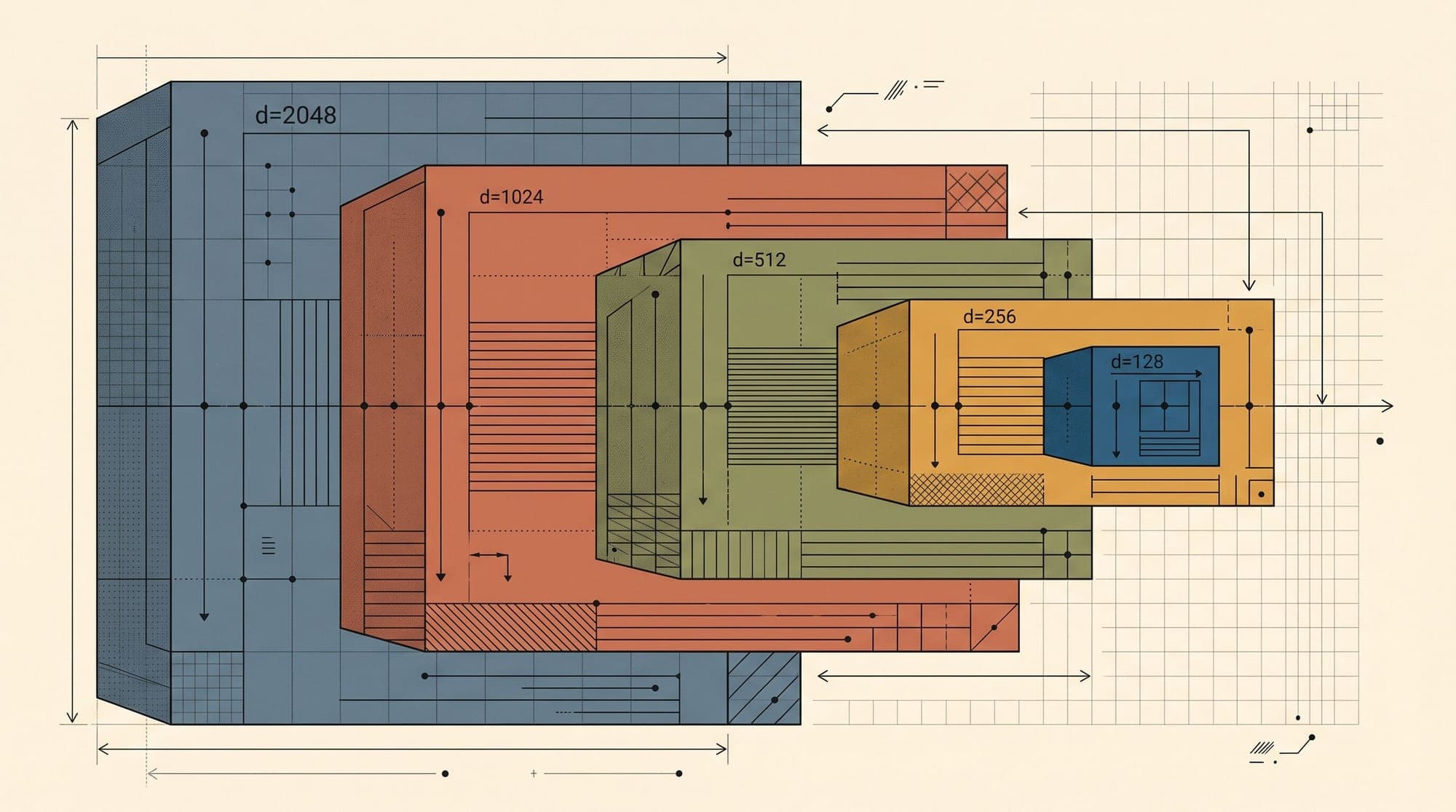
Matryoshka Representation Learning (MRL): Mathematical Foundations, Multi-Scale Loss Optimization, and Adaptive Vector Retrieval

Matryoshka Representation Learning (MRL) has become the standard architectural foundation for modern dense text embeddings. Introduced by Kusupati et al. at NeurIPS 2022 and subsequently deployed across frontier embedding models like OpenAI text-embedding-3, Nomic Embed, and BAAI BGE-M3, MRL solves a structural inefficiency in vector retrieval: the rigid coupling between embedding dimensionality, memory consumption, and semantic fidelity.

Traditional dense encoders project arbitrary text sequences into a fixed-dimensional vector space $\mathbb{R}^d$ (typically $d \in \{768, 1536, 3072\}$). While high dimensionality enables fine-grained semantic discrimination, it imposes prohibitive hardware costs on large-scale retrieval systems. MRL alters the training objective so that a single forward pass produces nested sub-vectors of varying dimensionalities, each independently capable of high-accuracy semantic retrieval.

The Fixed-Dimensional Bottleneck in Vector Retrieval

Modern retrieval-augmented generation (RAG) and dense search pipelines rely on embedding models to map queries and documents into dense metric spaces where semantic similarity corresponds to inner product or cosine distance.

In a standard deployment with $N$ documents and vector dimension $d$, the raw uncompressed vector storage footprint in 32-bit floating-point (FP32) is:

$$\text{RAM}_{\text{raw}} = N \times d \times 4 \text{ bytes}$$

For an enterprise corpus of $N = 10^8$ documents represented by 1536-dimensional embeddings:

$$\text{RAM}_{\text{raw}} = 10^8 \times 1536 \times 4 \text{ bytes} \approx 614.4 \text{ GB}$$

When building approximate nearest neighbor (ANN) graph indices such as Hierarchical Navigable Small World (HNSW), indexing overhead adds an additional $1.5\times$ to $2.0\times$ memory multiplier for graph edges and metadata, pushing RAM requirements beyond 1 TB.

Furthermore, the computational complexity of exhaustive or cluster-based distance comparisons scales linearly with dimension $d$:

$$\mathcal{O}(d) \text{ operations per vector comparison}$$

Historically, system designers faced an unyielding trade-off: deploy smaller embedding models (e.g., $d=256$ or $d=384$) and sacrifice retrieval precision across complex domains, or deploy large models ($d=1536$ or $d=3072$) and incur severe RAM, bandwidth, and latency penalties.

Contrastive Representation Learning and InfoNCE

Dense sentence encoders are trained using contrastive learning objectives on paired text corpora (e.g., query-document pairs, question-answer pairs, or natural language inference hypotheses). The core mechanism aligns positive pairs while dispersing negative pairs across the surface of a unit hypersphere $\mathcal{S}^{d-1}$.

Given a batch of $B$ query-passage pairs $\{(q_i, p_i^+)\}_{i=1}^B$ and an optional set of mined hard negatives $\{p_{i,k}^-\}_{k=1}^K$, the encoder generates normalized dense vectors $u_i = f_\theta(q_i) / \|f_\theta(q_i)\|_2$ and $v_i^+ = f_\theta(p_i^+) / \|f_\theta(p_i^+)\|_2$.

The objective is optimized via the InfoNCE loss function (introduced by van den Oord et al., 2018):

$$\mathcal{L}_{\text{InfoNCE}}(u_i, v_i^+) = -\log \frac{\exp\left(\frac{u_i^\top v_i^+}{\tau}\right)}{\exp\left(\frac{u_i^\top v_i^+}{\tau}\right) + \sum_{j \neq i}^B \exp\left(\frac{u_i^\top v_j^+}{\tau}\right) + \sum_{k=1}^K \exp\left(\frac{u_i^\top v_{i,k}^-}{\tau}\right)}$$

where $\tau > 0$ denotes the temperature hyperparameter.

Contrastive Hypersphere Optimization (Wang & Isola, 2020)
┌────────────────────────────────────────────────────────┐
│                      Unit Hypersphere S^(d-1)           │
│                                                        │
│         [q_i] ───(pull: Alignment)───> [p_i^+]         │
│           │                                            │
│           │                                            │
│       (push: Uniformity)                          │
│           │                                            │
│           ▼                                            │
│        [p_j^+] (in-batch) / [p_{i,k}^-] (hard negative)│
└────────────────────────────────────────────────────────┘

Alignment and Uniformity Dynamics

Wang and Isola (ICML 2020) demonstrated that contrastive optimization decomposes asymptotically into two concurrent geometric properties:

1. Alignment: Positive pairs should map to nearby features, minimizing expected distance:

$$\mathcal{L}_{\text{align}} \triangleq \mathbb{E}_{(x, x^+) \sim p_{\text{pos}}} \left[ \|f(x) - f(x^+)\|_2^\alpha \right] \quad (\alpha > 0)$$

1. Uniformity: The feature distribution should preserve maximal information by distributing uniformly over the unit hypersphere:

$$\mathcal{L}_{\text{uniform}} \triangleq \log \mathbb{E}_{x, y \stackrel{\text{i.i.d.}}{\sim} p_{\text{data}}} \left[ e^{-t \|f(x) - f(y)\|_2^2} \right] \quad (t > 0)$$

The temperature parameter $\tau$ dictates the hardness-aware penalty: small values of $\tau$ heavily penalize the closest negative points, preventing dimensional collapse and enforcing isotropic coverage across the sphere.

In unsupervised frameworks like SimCSE (Gao et al., 2021), the positive pair $(q_i, p_i^+)$ is synthesized by passing the exact same input sentence through the encoder twice with different standard dropout masks ($\Delta p = 0.1$). In supervised frameworks, positive pairs are augmented with mined hard negatives from BM25 or dense retrieval stages.

Matryoshka Representation Learning Formulation

In a standard neural encoder, features are distributed arbitrarily across all $d$ dimensions. Truncating a standard 1536-dimensional embedding down to 128 dimensions collapses retrieval performance because critical semantic variance is scattered non-linearly across the full coordinate basis.

Matryoshka Representation Learning (MRL), introduced by Kusupati et al. (2022), forces the network to order feature importance hierarchically. Like Russian nesting dolls (Matryoshka), smaller sub-vectors are nested within larger ones, with each prefix containing a self-sufficient semantic representation.

Nested Embedding Structure in MRL
┌───────────────────────────────────────────────────────────────────┐
│ d_1 = 64  │ Broad semantic topic, coarse categorization          │
├───────────┴─────────────────┐                                     │
│ d_2 = 256                   │ Intermediate semantic context       │
├─────────────────────────────┴───────────────────────┐             │
│ d_3 = 768                                           │ Fine nuance │
├─────────────────────────────────────────────────────┴─────────────┤
│ d_4 = 1536 (Full Vector)  Exact syntactic & entity-level details  │
└───────────────────────────────────────────────────────────────────┘

The Multi-Scale Loss Objective

Let $\mathcal{M} = \{d_1, d_2, \dots, d_K\}$ be an ordered set of target representation sizes such that:

$$d_1 < d_2 < \dots < d_K = d$$

A typical choice for a $d=1536$ model is $\mathcal{M} = \{64, 128, 256, 512, 1024, 1536\}$.

For each dimension $m \in \mathcal{M}$, we extract the prefix slice of the raw unnormalized representation vector $z = f_\theta(x) \in \mathbb{R}^d$:

$$z_{1:m} = \left[ z^{(1)}, z^{(2)}, \dots, z^{(m)} \right] \in \mathbb{R}^m$$

The MRL training loss is the weighted sum of contrastive losses computed over all nested dimensions simultaneously:

$$\mathcal{L}_{\text{MRL}} = \sum_{m \in \mathcal{M}} c_m \mathcal{L}_{\text{InfoNCE}}^{(m)}\left( \hat{u}_{1:m}, \hat{v}_{1:m}^+ \right)$$

where $c_m > 0$ represents the loss weight for dimension $m$ (frequently set uniformly as $c_m = \frac{1}{|\mathcal{M}|}$), and $\hat{u}_{1:m}$ is the independently normalized prefix vector.

The Slice-Then-Normalize Rule

A crucial mathematical constraint in MRL is the ordering of truncation and normalization.

If a full vector $z \in \mathbb{R}^d$ is first normalized to unit length $\|z\|_2 = 1$, slicing its prefix produces a sub-vector whose Euclidean norm is strictly less than one:

$$\|z_{1:m}\|_2 = \sqrt{\sum_{i=1}^m \left(z^{(i)}\right)^2} \le \|z\|_2 = 1$$

Computing cosine similarity on unnormalized or pre-normalized truncated slices degrades the angular geometry of the sub-space. Under MRL, the representation must be sliced first, then L2-normalized:

$$\hat{z}_{1:m} = \frac{z_{1:m}}{\|z_{1:m}\|_2} = \frac{\left[ z^{(1)}, z^{(2)}, \dots, z^{(m)} \right]}{\sqrt{\sum_{j=1}^m \left(z^{(j)}\right)^2}}$$

Every sub-vector $\hat{z}_{1:m}$ is mapped to its own unit hypersphere $\mathcal{S}^{m-1}$, preserving strict cosine distance equivalence during downstream indexing:

$$\text{sim}(\hat{u}_{1:m}, \hat{v}_{1:m}) = \hat{u}_{1:m}^\top \hat{v}_{1:m} \in [-1, 1]$$

Why MRL Outperforms Post-Hoc Dimension Reduction

A common question is why MRL is necessary when post-processing techniques like Principal Component Analysis (PCA) or Singular Value Decomposition (SVD) can reduce dimensionality after training.

PCA identifies the orthogonal directions of maximal variance in static feature space:

$$Z = U \Sigma V^\top \implies Z_k = U_k \Sigma_k$$

However, post-hoc linear projection fails for three reasons:

1. Non-Linear Manifolds: Transformer representations reside on complex non-linear manifolds. Linear orthogonal projections ignore non-linear semantic boundaries established by attention layers.
2. Contrastive Objective Mismatch: PCA maximizes total reconstruction variance $\text{Tr}(\text{Var}(Z))$, not class separation or ranking order. Directions of high variance frequently capture lexical artifacts rather than semantic relevance.
3. End-to-End Gradient Propagation: MRL backpropagates gradients from all nested dimensions simultaneously into the Transformer weights:

$$\frac{\partial \mathcal{L}_{\text{MRL}}}{\partial \theta} = \sum_{m \in \mathcal{M}} c_m \frac{\partial \mathcal{L}^{(m)}}{\partial \hat{z}_{1:m}} \frac{\partial \hat{z}_{1:m}}{\partial \theta}$$

This forces the Transformer backbone to pack the highest-entropy, most discriminative semantic signals into the earliest coordinate indices ($1 \dots d_1$), while allocating subsequent dimensions ($d_1+1 \dots d$) to residual variance and fine-grained distinctions.

Gradient Flow in Matryoshka Multi-Scale Optimization
┌────────────────────────────────────────────────────────┐
│ Input Tokens: [x_1, x_2, ..., x_L]                     │
│                        │                               │
│              Transformer Encoder (θ)                   │
│                        │                               │
│         Dense Hidden State z in R^d (d=1536)           │
│         ┌───────────┬───────────┬───────────┐          │
│         │  z_(1:64) │ z_(1:256) │ z_(1:1536)│          │
│         └─────┬─────┴─────┬─────┴─────┬─────┘          │
│               │           │           │                │
│            L2-Norm     L2-Norm     L2-Norm             │
│               │           │           │                │
│            InfoNCE     InfoNCE     InfoNCE             │
│            Loss L_64   Loss L_256  Loss L_1536         │
│               │           │           │                │
│               └─────┬─────┴───────────┘                │
│                     ▼                                  │
│           Total L_MRL Backpropagation                  │
└────────────────────────────────────────────────────────┘

Production Systems: Adaptive Funnel Search and Quantization Synergy

The true utility of MRL is realized in tiered, multi-stage retrieval architectures (often termed cascading search or funnel retrieval).

Instead of searching a billion 1536-dimensional vectors with high computational overhead, systems decouple candidate generation from candidate reranking.

Two-Stage Funnel Search Pipeline

1. Stage 1: Coarse Shortlisting (Sub-Vector Search)

• All $N$ corpus documents are indexed using a low-dimensional MRL slice (e.g., $d_1 = 64$ or $d_2 = 128$).
• A low-dimensional HNSW index or inverted file index (IVF) executes approximate nearest neighbor search over the query slice $\hat{u}_{1:64}$.
• The top $K$ candidates (e.g., $K = 100$) are retrieved in milliseconds with minimal memory bandwidth consumption.

1. Stage 2: Fine-Grained Rescoring (Full-Vector Refinement)

• The system retrieves the full $d_K = 1536$ representation for only the top $K$ shortlisted documents from secondary NVMe storage or compressed memory.
• Exact inner products $\hat{u}_{1:1536}^\top \hat{v}_{1:1536}$ are evaluated across the $K$ candidates to produce the final top-10 ranking.

Two-Stage Funnel Search Workflow
┌────────────────────────────────────────────────────────┐
│ Query q  ───>  MRL Encoder  ───>  u in R^1536          │
│                                    │                   │
│           Extract u_(1:64) ────────┼──────────────┐    │
│                  │                                │    │
│                  ▼                                │    │
│        [ Stage 1: Fast ANN ]                      │    │
│        Search 100M docs in R^64                   │    │
│        Output: Top K=100 Candidates               │    │
│                  │                                │    │
│                  ▼                                │    │
│        [ Stage 2: Exact Rescore ]                 │    │
│        Fetch 100 full vectors in R^1536 <─────────┘    │
│        Output: Top 10 Final Results                    │
└────────────────────────────────────────────────────────┘

Empirical Retrieval Efficiency

Evaluations across the Massive Text Embedding Benchmark (MTEB) demonstrate the efficiency frontier established by MRL:

• Truncating a 1536-dimensional MRL embedding to 256 dimensions ($6\times$ reduction in size) preserves over $98.5\%$ of the full-dimensional NDCG@10 retrieval performance.
• Truncating to 64 dimensions ($24\times$ reduction in size) retains over $94\%\text{--}96\%$ of retrieval precision.
• Funnel retrieval (64-dim shortlist followed by 1536-dim rescore) matches $99.9\%$ of full-dimensional search accuracy while reducing total vector search latency by up to $14\times$.

Compounding with Binary and Scalar Quantization

MRL compounds multiplicatively with vector quantization methods:

• 1-Bit Binary Quantization: Taking the sign bit $\text{sign}(\hat{z}_{1:m}) \in \{-1, +1\}^m$ packs each dimension into a single bit. A 128-dimensional vector occupies just 16 bytes (128 bits). Similarity is evaluated using hardware-accelerated bitwise XOR and POPCNT instructions.
• Int8 Scalar Quantization: Quantizing float values to 8-bit integers achieves an immediate $4\times$ memory reduction with negligible precision loss.

Combining a 128-dimensional MRL slice with 1-bit binary quantization yields a $384\times$ reduction in storage compared to a 1536-dimensional FP32 baseline ($1536 \times 4 = 6144$ bytes vs. $16$ bytes).

Reference PyTorch Implementation

Below is a complete reference implementation of an MRL contrastive loss module supporting arbitrary nested dimensions and in-batch negative InfoNCE:

import torch
import torch.nn as nn
import torch.nn.functional as F

class MatryoshkaContrastiveLoss(nn.Module):
    """
    Matryoshka Representation Learning (MRL) Contrastive Loss.
    Wraps multi-scale InfoNCE loss over nested embedding dimensions.
    """
    def __init__(
        self,
        dimensions: list[int] = [64, 128, 256, 512, 1024, 1536],
        temperature: float = 0.05,
        weights: list[float] | None = None,
    ):
        super().__init__()
        self.dimensions = sorted(dimensions)
        self.temperature = temperature
        
        if weights is not None:
            assert len(weights) == len(dimensions)
            total = sum(weights)
            self.weights = [w / total for w in weights]
        else:
            self.weights = [1.0 / len(dimensions)] * len(dimensions)

    def forward(
        self,
        query_embeddings: torch.Tensor,
        passage_embeddings: torch.Tensor,
    ) -> torch.Tensor:
        """
        Args:
            query_embeddings: Unnormalized Tensor of shape (batch_size, full_dim)
            passage_embeddings: Unnormalized Tensor of shape (batch_size, full_dim)
        Returns:
            Scalar loss averaged over all Matryoshka dimensions.
        """
        total_loss = torch.tensor(0.0, device=query_embeddings.device)
        batch_size = query_embeddings.size(0)
        labels = torch.arange(batch_size, device=query_embeddings.device)

        for dim, weight in zip(self.dimensions, self.weights):
            # 1. Slice prefix sub-vectors
            q_slice = query_embeddings[:, :dim]
            p_slice = passage_embeddings[:, :dim]

            # 2. Slice-then-normalize to unit hypersphere S^(dim-1)
            q_norm = F.normalize(q_slice, p=2, dim=-1)
            p_norm = F.normalize(p_slice, p=2, dim=-1)

            # 3. Compute in-batch cosine similarity logits
            similarity_matrix = torch.matmul(q_norm, p_norm.t()) / self.temperature

            # 4. InfoNCE cross-entropy loss
            loss_dim = F.cross_entropy(similarity_matrix, labels)
            total_loss += weight * loss_dim

        return total_loss

Summary and Architectural Impact

Matryoshka Representation Learning transforms dense vector embeddings from static, monolithic representations into dynamic, multi-resolution feature hierarchies. By optimizing nested sub-vector losses jointly during training, MRL enables:

1. Granular Elasticity: Developers can choose arbitrary embedding sizes (e.g., 64d, 256d, 1536d) at inference time from a single unified checkpoint without re-indexing or retraining.
2. Infrastructure Cost Reduction: High-throughput vector search engines leverage coarse-to-fine funnel pipelines to slash index RAM requirements by over $90\%$ while preserving top-tier retrieval accuracy.
3. Synergy with Hardware Acceleration: Low-dimensional prefixes integrate seamlessly with binary quantization and SIMD bitwise instructions for sub-millisecond retrieval across massive corpora.

Sources

• Kusupati, A., Bhatt, G., Rege, A., et al. (2022). Matryoshka Representation Learning. Advances in Neural Information Processing Systems (NeurIPS 2022).
• Gao, T., Yao, X., & Chen, D. (2021). SimCSE: Simple Contrastive Learning of Sentence Embeddings. Empirical Methods in Natural Language Processing (EMNLP 2021).
• Wang, T., & Isola, P. (2020). Understanding Contrastive Representation Learning through Alignment and Uniformity on the Hypersphere. International Conference on Machine Learning (ICML 2020).
• van den Oord, A., Li, Y., & Vinyals, O. (2018). Representation Learning with Contrastive Predictive Coding. arXiv:1807.03748.
• OpenAI (2024). New Embedding Models and API Updates: Matryoshka Representation Learning in text-embedding-3.
• Nomic AI (2024). Nomic Embed: Training Open-Source MRL Embeddings.
• Muennighoff, N., Tazi, N., Magne, L., & Reimers, N. (2023). MTEB: Massive Text Embedding Benchmark. EACL 2023.