Jacobi and Lookahead Decoding: How Parallel Fixed-Point Iteration Accelerates Autoregressive Inference Without Draft Models

Standard autoregressive generation in large language models operates as a strictly sequential process. To generate a sequence of $K$ tokens, an inference engine must execute $K$ successive forward passes through the network. In single-request serving regimes (batch size 1), each forward pass is heavily memory-bandwidth bound: the GPU must stream billions of model parameters from High Bandwidth Memory (HBM) into on-chip SRAM to process a single token, leaving tensor compute cores severely underutilized.

Speculative decoding mitigates this memory bottleneck by introducing a smaller auxiliary draft model to propose token candidates verified in parallel by the target LLM. However, draft-based speculative decoding introduces substantial engineering friction: deploying and synchronizing two models, managing dual key-value (KV) caches, aligning vocabulary tokenizers, and absorbing extra GPU memory overhead.

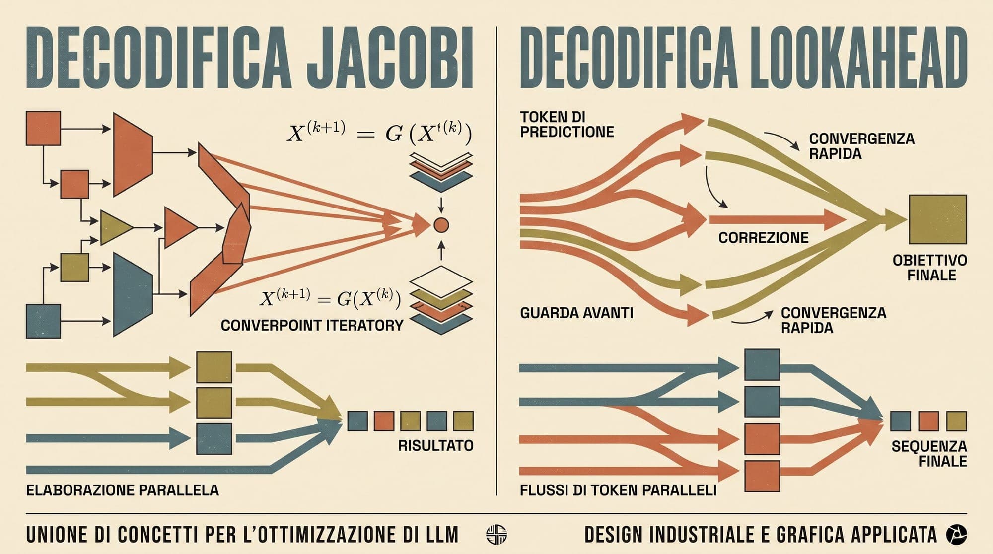
Jacobi decoding and Lookahead decoding offer a fundamentally different paradigm: parallelizing token generation directly on the target LLM without auxiliary models, architectural modifications, or secondary training. By reformulating autoregressive generation as solving a system of non-linear equations via fixed-point iteration, these techniques trade idle GPU compute for reduced latency while maintaining mathematical equivalence to standard greedy decoding.

Formulating Autoregressive Decoding as a Fixed-Point Problem

In standard greedy autoregressive decoding, each token $y_i$ is determined conditioned on all preceding tokens $y_{<i}$ and prompt context $x$:

$$y_i = \arg\max_{v \in \mathcal{V}} P(Y_i = v \mid x, y_1, y_2, \dots, y_{i-1})$$

For a target block of $K$ future tokens $\mathbf{y} = [y_1, y_2, \dots, y_K]^\top$, this dependency defines a lower-triangular non-linear system:

$$y_1 = f_1(x)$$ $$y_2 = f_2(x, y_1)$$ $$y_3 = f_3(x, y_1, y_2)$$ $$y_K = f_K(x, y_1, y_2, \dots, y_{K-1})$$

In vector notation, this system can be expressed as a fixed-point equation $\mathbf{y} = F(\mathbf{y})$, where $F: \mathcal{V}^K \to \mathcal{V}^K$ is the multi-token forward evaluation operator defined by the causal transformer.

The Jacobi Fixed-Point Iteration

Classical numerical linear algebra solves fixed-point systems $\mathbf{y} = F(\mathbf{y})$ using Jacobi iteration. In Jacobi decoding, as formalized by Santilli et al. (2023), the model starts from an initial guess vector $\mathbf{y}^{(0)} = [y_1^{(0)}, y_2^{(0)}, \dots, y_K^{(0)}]^\top$ (such as padding tokens or repeated prompt tokens).

At each iteration step $t \ge 0$, the transformer processes all $K$ token positions simultaneously in a single forward pass:

$$y_i^{(t+1)} = f_i(x, y_1^{(t)}, y_2^{(t)}, \dots, y_{i-1}^{(t)})$$

Because the underlying system is strictly lower-triangular, Jacobi decoding possesses a deterministic convergence guarantee:

1. Step 1: The first token $y_1^{(1)} = f_1(x)$ depends only on the context $x$ and converges immediately to the exact autoregressive greedy token.
2. Step 2: The second token $y_2^{(2)} = f_2(x, y_1^{(1)})$ receives the exact converged value of $y_1$ and reaches its true fixed point.
3. Step $K$: By mathematical induction, all $K$ variables $\mathbf{y}^{(K)}$ are guaranteed to reach their exact autoregressive fixed point in at most $K$ iteration steps.

When local syntactic or semantic patterns are predictable, multiple positions often converge simultaneously in far fewer than $K$ steps. For instance, common phrases or boilerplate code constructs can settle to their fixed points within 2 to 3 Jacobi iterations.

Why Pure Jacobi Decoding Fails in Production

Despite the theoretical appeal of parallel fixed-point solving, vanilla Jacobi decoding rarely delivers wall-clock speedups in practical LLM serving. Empirical investigations in Fu et al. (2024) identified three fundamental bottlenecks in pure Jacobi iteration:

1. Unstable Intermediate States: Tokens generated at position $i$ during early iterations are conditioned on unconverged, noisy guesses from positions $j < i$. When an upstream token flips during a later iteration, it invalidates downstream tokens, causing cascading recomputations.
2. Position Displacement: During intermediate steps, Jacobi iterations frequently generate valid multi-token sequences at incorrect positional offsets. In vanilla Jacobi decoding, these correctly predicted tokens are discarded if their exact sequence indices do not match the target vector.
3. Trajectory Overwriting: A subsequent Jacobi iteration may overwrite a correct n-gram generated in an earlier step before the fixed-point solver reaches that position.
4. Low Token-Per-Step Yield: In open-ended language generation, pure Jacobi iteration averages only 1.1 to 1.3 accepted tokens per forward pass. The minor reduction in step count fails to offset the additional FLOPs and KV cache management overhead.

Lookahead Decoding: Converting Trajectories into N-Gram Candidates

To overcome the fragility of pure Jacobi decoding, Fu et al. (2024) developed Lookahead Decoding (introduced via LMSYS Organization). Rather than waiting for a rigid $K$-token vector to converge monolithically, Lookahead Decoding treats the Jacobi iteration trajectory as an online generator of candidate n-grams.

In Lookahead Decoding, each decoding step divides model execution into two parallel branches executed in a single forward pass:

1. The Lookahead Branch

The lookahead branch maintains a fixed-size 2D window of dimensions $W \times (N-1)$, where $W$ represents the sequence window size and $N$ represents the target n-gram length. The two axes correspond to:

• Sequence Axis: Future token positions extending from the current generation frontier.
• Iteration Axis: Successive Jacobi iteration steps across time.

As the lookahead branch executes Jacobi updates across this 2D window, it generates a continuous stream of candidate n-grams across iterations. Instead of discarding intermediate noisy states, the engine extracts and caches all distinct n-grams produced along the Jacobi trajectory.

2. The Verification Branch

The verification branch selects promising candidate n-grams from the trajectory cache and verifies them in parallel against the current sequence prefix.

If the verification branch validates a candidate $N$-gram $(y_1, y_2, \dots, y_M)$ where $M \le N$, all $M$ tokens are accepted simultaneously in that single step. The generation frontier advances by $M$ tokens, and the lookahead window slides forward to cover the new horizon.

Attention Mask Construction for Dual-Branch Execution

Executing the lookahead and verification branches in a single forward pass requires a structured 2D attention mask to preserve causal isolation:

• Prompt and Prefix Tokens: Attend causally only to preceding prefix tokens.
• Verification Candidates: Flattened into a candidate tree where each candidate token attends to the verified prefix and its own intra-candidate ancestors. Candidates cannot attend across sibling candidate branches.
• Lookahead Tokens: Attend to the prefix and their respective local Jacobi window states without leaking information into the verification branch.

By utilizing custom causal tree masks, both n-gram generation (lookahead) and candidate validation (verification) run simultaneously in one batched kernel launch.

Arithmetic Intensity and FLOP Redundancy

The efficiency of Lookahead Decoding stems from the arithmetic characteristics of modern GPU hardware. In standard autoregressive serving at batch size 1, GPU compute utilization is typically under 10%. Memory bandwidth dictates latency: loading weights for a 70-billion-parameter model takes roughly 10 to 15 milliseconds regardless of whether the model evaluates 1 token or 64 tokens.

Lookahead Decoding exploits this FLOP redundancy:

• FLOP Budget: Processing $W \times (N-1)$ lookahead tokens plus $G \times (N-1)$ verification tokens increases arithmetic intensity per step.
• Latency Invariance: Because the total number of candidate tokens remains well within the memory-bound threshold of modern GPU tensor cores, a forward pass evaluating 30 to 60 candidate tokens takes nearly identical wall-clock time as a single-token autoregressive step.
• Step Compression: Fu et al. (2024) demonstrated that Lookahead Decoding follows a logarithmic scaling relationship: an exponential increase in window size $W$ yields a linear reduction in total decoding steps.

Because verification enforces exact greedy equivalence against the base model logits, the generated text is mathematically identical to standard autoregressive generation with zero distributional shift or output degradation.

Architectural Comparison: Speculative, Jacobi, and Lookahead Decoding

The core differences across parallel decoding strategies include:

• Standard Autoregressive Decoding:
• Auxiliary models required: None.
• Training or fine-tuning: None.
• GPU memory overhead: Baseline (single model and single KV cache).
• Mathematical equivalence: Exact greedy baseline.
• Typical speedup: 1.0x (baseline).
• Operating regime: General serving.
• Speculative Decoding (Draft Model):
• Auxiliary models required: Yes (a smaller draft LLM).
• Training or fine-tuning: Requires aligned tokenizer and draft model training.
• GPU memory overhead: High (two active models in VRAM, dual KV caches).
• Mathematical equivalence: Exact (via modified rejection sampling).
• Typical speedup: 1.8x to 2.8x.
• Operating regime: Low batch size, memory-bandwidth bound.
• Vanilla Jacobi Decoding:
• Auxiliary models required: None.
• Training or fine-tuning: None.
• GPU memory overhead: Minimal (small trajectory buffer).
• Mathematical equivalence: Exact at full fixed-point convergence.
• Typical speedup: 1.0x to 1.1x.
• Operating regime: Academic interest, low practical speedup.
• Lookahead Decoding:
• Auxiliary models required: None.
• Training or fine-tuning: None (operates zero-shot on any autoregressive LLM).
• GPU memory overhead: Low (2D trajectory window and candidate n-gram cache).
• Mathematical equivalence: Exact greedy equivalence.
• Typical speedup: 1.5x to 2.3x.
• Operating regime: Low batch size, memory-bandwidth bound.

Further Developments: Jacobi Forcing and Iteration Training

While training-free Lookahead Decoding accelerates inference on off-the-shelf checkpoints, recent research explores training models specifically to improve Jacobi trajectory convergence.

Snowflake Engineering (2024) introduced Jacobi Forcing, a post-training technique that exposes models to intermediate Jacobi trajectories during fine-tuning. By training intermediate layers to map noisy Jacobi states directly to their final fixed-point targets, Jacobi Forcing accelerates convergence, increasing the average accepted tokens per iteration without requiring auxiliary draft architectures.

Conclusion

Jacobi and Lookahead Decoding demonstrate that the sequential bottleneck of autoregressive LLM inference is not an immutable constraint. By reframing token generation as fixed-point iteration and capturing n-gram candidates across iterative trajectories, inference engines can harvest idle GPU compute to reduce serving latency while eliminating the operational complexity of auxiliary draft models.

Sources

• Fu, Y., Bailis, P., Stoica, I., & Zhang, H. (2024). Break the Sequential Dependency of LLM Inference Using Lookahead Decoding. ICML 2024.
• Santilli, A., Severino, S., Postolache, E., Maiorca, V., Mancusi, M., Marin, R., & Rodola, E. (2023). Accelerating Transformer Inference for Translation via Parallel Decoding. ACL 2023.
• Leviathan, Y., Kalman, M., & Matias, Y. (2023). Fast Inference from Transformers via Speculative Decoding. ICML 2023.
• LMSYS Organization. (2023). Break the Sequential Dependency of LLM Inference Using Lookahead Decoding.
• Snowflake Engineering. (2024). Fast and More Accurate Causal Parallel Decoding Using Jacobi Forcing.