Grouped-Query Attention (GQA) and Multi-Query Attention (MQA): Mathematical Foundations, KV Cache Memory Reduction, and Arithmetic Intensity in Transformer Serving

Autoregressive generation in large language models exhibits an asymmetric computational profile between initial prompt processing (prefill) and subsequent incremental generation (decode). While prefill parallelizes across all prompt tokens and achieves high compute utilization on modern tensor accelerators, token-by-token decoding is heavily memory-bandwidth bound. Each generated token requires reading the entire accumulated Key-Value (KV) cache from High Bandwidth Memory (HBM) into on-chip SRAM to compute attention against a single query token.

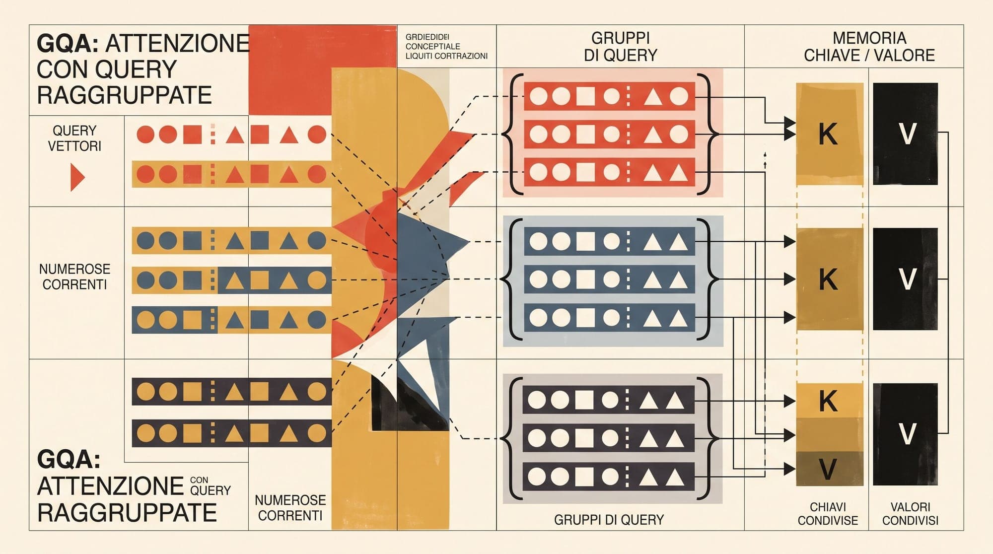
Standard Multi-Head Attention (MHA) allocates independent key and value projections for every attention head, causing the KV cache footprint and memory traffic to scale linearly with the number of query heads. To alleviate this memory wall, Multi-Query Attention (MQA) introduced extreme compression by sharing a single key-value head across all query heads, but often suffered from capacity degradation and optimization instability. Grouped-Query Attention (GQA) formalizes an intermediate parameterization where query heads are partitioned into groups that share key-value projections.

Standard Multi-Head Attention (MHA):
Query Heads (H): [ Q1 ] [ Q2 ] [ Q3 ] [ Q4 ] [ Q5 ] [ Q6 ] [ Q7 ] [ Q8 ]
Key Heads   (H): [ K1 ] [ K2 ] [ K3 ] [ K4 ] [ K5 ] [ K6 ] [ K7 ] [ K8 ]
Value Heads (H): [ V1 ] [ V2 ] [ V3 ] [ V4 ] [ V5 ] [ V6 ] [ V7 ] [ V8 ]

Grouped-Query Attention (GQA, G=2, Group Size=4):
Query Heads (H): [ Q1   Q2   Q3   Q4 ]   [ Q5   Q6   Q7   Q8 ]
Key Heads   (G): [        K1         ]   [        K2         ]
Value Heads (G): [        V1         ]   [        V2         ]

Multi-Query Attention (MQA, G=1):
Query Heads (H): [ Q1   Q2   Q3   Q4   Q5   Q6   Q7   Q8 ]
Key Heads   (1): [                  K1                  ]
Value Heads (1): [                  V1                  ]

Mathematical Formulation of Attention Variants

Consider a Transformer hidden state $X \in \mathbb{R}^{B \times N \times d}$ , where $B$ denotes batch size, $N$ denotes sequence length, and $d$ represents the model hidden dimension. Let $H$ be the number of query attention heads, and $d_k = d / H$ be the per-head projection dimension.

1. Multi-Head Attention (MHA)

In standard MHA (Vaswani et al., 2017), linear projection weight matrices transform input representations into query, key, and value tensors:

$W_Q \in \mathbb{R}^{d \times (H \cdot d_k)}, \quad W_K \in \mathbb{R}^{d \times (H \cdot d_k)}, \quad W_V \in \mathbb{R}^{d \times (H \cdot d_k)}, \quad W_O \in \mathbb{R}^{(H \cdot d_k) \times d}$

For each head $h \in \{1, \dots, H\}$ :

$Q_h = X W_{Q, h}, \quad K_h = X W_{K, h}, \quad V_h = X W_{V, h}$

$\text{Head}_h = \text{softmax}\left( \frac{Q_h K_h^T}{\sqrt{d_k}} \right) V_h$

$\text{MHA}(X) = \text{Concat}(\text{Head}_1, \dots, \text{Head}_H) W_O$

Every query head $h$ maintains its own dedicated key $K_h$ and value $V_h$ representation in GPU memory.

2. Multi-Query Attention (MQA)

Introduced by Shazeer (2019), MQA collapses the key and value projections into a single shared head ( $G = 1$ ):

$W_Q \in \mathbb{R}^{d \times (H \cdot d_k)}, \quad W_K \in \mathbb{R}^{d \times d_k}, \quad W_V \in \mathbb{R}^{d \times d_k}$

The projection tensors produce $H$ distinct query matrices but only single key and value matrices:

$Q_h = X W_{Q, h} \in \mathbb{R}^{B \times N \times d_k}, \quad K = X W_K \in \mathbb{R}^{B \times N \times d_k}, \quad V = X W_V \in \mathbb{R}^{B \times N \times d_k}$

For each query head $h \in \{1, \dots, H\}$ , attention is computed against the shared $K$ and $V$ :

$\text{Head}_h = \text{softmax}\left( \frac{Q_h K^T}{\sqrt{d_k}} \right) V$

$\text{MQA}(X) = \text{Concat}(\text{Head}_1, \dots, \text{Head}_H) W_O$

While MQA reduces the KV cache size by a factor of $H$ , the representational bottleneck can lead to performance degradation on reasoning-intensive benchmarks, synthetic retrieval, and long-context association tasks.

3. Grouped-Query Attention (GQA)

Introduced by Ainslie et al. (2023), Grouped-Query Attention partitions the $H$ query heads into $G$ uniform groups, where $1 < G < H$ . Each group contains $M = H / G$ query heads that share a single key-value head pair:

$W_Q \in \mathbb{R}^{d \times (H \cdot d_k)}, \quad W_K \in \mathbb{R}^{d \times (G \cdot d_k)}, \quad W_V \in \mathbb{R}^{d \times (G \cdot d_k)}$

Let group index $g(h) = \lfloor (h - 1) / M \rfloor + 1 \in \{1, \dots, G\}$ . The projections yield:

$Q_h = X W_{Q, h}, \quad K_g = X W_{K, g}, \quad V_g = X W_{V, g}$

For query head $h$ , attention is evaluated with the corresponding group key-value tensors:

$\text{Head}_h = \text{softmax}\left( \frac{Q_h K_{g(h)}^T}{\sqrt{d_k}} \right) V_{g(h)}$

$\text{GQA}(X) = \text{Concat}(\text{Head}_1, \dots, \text{Head}_H) W_O$

When $G = H$ , GQA is identical to standard MHA. When $G = 1$ , GQA reduces to MQA. Typical production configurations set $G = 8$ with $H = 32$ or $H = 64$ , providing a 4x to 8x reduction in key-value memory while maintaining near-perfect benchmark parity with MHA.

Architectural comparison of MHA, GQA, and MQA memory access patterns

Roofline Modeling and Arithmetic Intensity

To understand why GQA is the standard in modern LLM serving (e.g., Llama 2 and Llama 3), one must evaluate the operational arithmetic intensity during the autoregressive decode phase.

Decode Memory Traffic and Computational Complexity

In the decode phase, the model processes a single new token ( $N=1$ ) for a batch of $B$ concurrent requests across a context of length $S$ .

For a Transformer layer with $L$ layers:

Weight Matrix Memory Access:

Loading model weights requires reading the parameter matrices from HBM once per generated token: $\text{Bytes}_{\text{weights}} \approx 2 \cdot P \quad (\text{for 16-bit precision})$ where $P$ is the parameter count.

KV Cache Memory Access:

For each token in the batch, the entire historical KV cache of length $S$ must be loaded from HBM into SRAM: $\text{Bytes}_{\text{KV}} = 2 \cdot B \cdot S \cdot G \cdot d_k \cdot \text{dtype\_bytes}$ where the factor 2 accounts for both keys and values.

Floating Point Operations (FLOPs):

The attention score computation $Q K^T$ and context aggregation $\text{Attn} \cdot V$ require: $\text{FLOPs}_{\text{attn}} = 4 \cdot B \cdot S \cdot H \cdot d_k$

Operational Intensity Calculation

Arithmetic intensity $\mathcal{I}$ is defined as the ratio of floating-point operations to memory bytes transferred across the memory bus:

$\mathcal{I}_{\text{attn}} = \frac{\text{FLOPs}_{\text{attn}}}{\text{Bytes}_{\text{KV}}} = \frac{4 \cdot B \cdot S \cdot H \cdot d_k}{2 \cdot B \cdot S \cdot G \cdot d_k \cdot 2} = \frac{H}{G} \quad \left[\frac{\text{FLOPs}}{\text{Byte}}\right] \quad (\text{for 16-bit / 2-byte floats})$

Under standard MHA ( $G = H$ ): $\mathcal{I}_{\text{attn, MHA}} = 1.0 \text{ FLOP/Byte}$

On an NVIDIA H100 SXM GPU (3.35 TB/s HBM3 memory bandwidth, 989 TFLOPS BF16 tensor core throughput), the hardware balance point (ridge point) occurs at:

$\mathcal{I}_{\text{hardware}} = \frac{989 \times 10^{12} \text{ FLOPs/s}}{3.35 \times 10^{12} \text{ Bytes/s}} \approx 295 \text{ FLOPs/Byte}$

Because $1.0 \ll 295$ , MHA decoding is severely bandwidth-bound. The tensor cores spend over 99% of cycles stalled waiting for KV cache bytes to stream from HBM.

Under GQA with $H = 64$ and $G = 8$ ( $H/G = 8$ ):

KV cache memory transfer is reduced by 87.5% (8x reduction).
Arithmetic intensity inside the attention kernel increases eightfold.
For a fixed GPU memory budget, the maximum serving batch size $B$ increases by up to 8x, directly scaling serving throughput.

Checkpoint Conversion and the Uptraining Recipe

A crucial contribution of Ainslie et al. (2023) was demonstrating that existing MHA checkpoints can be converted into GQA or MQA architectures without training from scratch.

1. Mean-Pooling Weight Transformation

To convert an MHA checkpoint with $H$ key and value heads into a GQA checkpoint with $G$ groups, the projection slices corresponding to each group are averaged:

$W_{K, g}^{\text{GQA}} = \frac{1}{|S_g|} \sum_{h \in S_g} W_{K, h}^{\text{MHA}}, \quad W_{V, g}^{\text{GQA}} = \frac{1}{|S_g|} \sum_{h \in S_g} W_{V, h}^{\text{MHA}}$

where $S_g = \{ (g-1)M + 1, \dots, gM \}$ represents the set of MHA head indices mapped to group $g$ .

Empirical evaluations showed that mean-pooling preserved substantial representation structure, outperforming first-head selection or random reinitialization.

2. Adaptation Pre-Training (Uptraining)

Following weight pooling, the model undergoes continued pre-training (uptraining) on approximately 5% of its original pre-training token budget. During uptraining:

The query projections adjust their attention geometry to align with the shared subspace of the grouped key-value heads.
GQA-8 (8 KV groups) achieved performance parity with the full MHA baseline across summarization (CNN/DailyMail, MultiNews), question answering (TriviaQA), and translation benchmarks (WMT14), while matching the high-throughput inference speed of MQA.

+------------------+-------------------+-------------------+-------------------+
| Architecture     | KV Cache Size     | Decode Bandwidth  | Benchmark Quality |
+------------------+-------------------+-------------------+-------------------+
| Multi-Head (MHA) | 100% (Baseline)   | High (Bottleneck) | Full Capacity     |
| Grouped (GQA-8)  | 12.5% to 25.0%    | Reduced (3-8x)    | ~100% of MHA      |
| Multi-Query(MQA) | 3.1% to 6.2%      | Minimal           | Slight Drop       |
+------------------+-------------------+-------------------+-------------------+

Architectural Evolution: GQA vs. Multi-Head Latent Attention (MLA)

While GQA has become the de facto standard across open-weight models (including Mistral 7B, Llama 3 8B/70B/405B, Qwen 2.5, and Gemma 2), architectural research has continued exploring KV cache compression.

DeepSeek-V2 and DeepSeek-V3 introduced Multi-Head Latent Attention (MLA), which compresses the KV cache through low-rank joint latent vectors:

$c_t^{KV} = W_{DKV} h_t \in \mathbb{R}^{d_c}$

where $d_c \ll H \cdot d_k$ . During generation, only the compressed latent vector $c_t^{KV}$ (along with a decoupled RoPE key) is cached in HBM. While MLA achieves even higher compression ratios than GQA, it requires matrix multiplications to project latents into per-head keys and values during computation, trading small compute overhead for maximum memory compression.

For general transformer architectures, GQA remains the standard because it requires zero decompression compute during kernel execution, seamlessly integrates with FlashAttention-2, FlashDecoding, and vLLM PagedAttention kernels, and enables multi-fold throughput scaling on enterprise inference clusters.