Generalized Advantage Estimation: How Exponential Weighting Balances Bias and Variance in Policy Optimization

Policy gradient algorithms form the theoretical backbone of modern policy optimization, ranging from continuous robotic control to reinforcement learning from human feedback (RLHF) in frontier large language models. A persistent challenge in policy optimization is variance: estimating the gradient of expected cumulative reward over stochastic trajectories generates high-variance Monte Carlo signals that require massive sample sizes and risk destabilizing gradient updates.

Generalized Advantage Estimation (GAE), introduced by John Schulman, Philipp Moritz, Sergey Levine, Michael I. Jordan, and Pieter Abbeel in 2015, provides a formal mathematical framework to balance bias and variance in advantage estimation. By constructing an exponentially weighted average of multi-step temporal difference residuals, GAE enables stable policy updates across complex, high-dimensional state spaces.

The Variance Problem in Policy Gradients

Under the policy gradient theorem established by Sutton et al. (1999), the gradient of the expected discounted return with respect to policy parameters theta is expressed as:

grad_theta J(theta) = E [ sum_{t=0}^T grad_theta log pi_theta(a_t | s_t) * Psi_t ]

The choice of the scalar multiplier Psi_t determines the variance and bias of the gradient estimator. Standard choices include:

1. Total trajectory return: Psi_t = sum_{t'=0}^T r_{t'}
2. Reward-to-go: Psi_t = sum_{t'=t}^T gamma^(t'-t) r_{t'}
3. State-action value function: Psi_t = Q^pi(s_t, a_t)
4. Advantage function: Psi_t = A^pi(s_t, a_t) = Q^pi(s_t, a_t) - V^pi(s_t)

Using raw trajectory returns or reward-to-go yields completely unbiased estimators, but the variance grows rapidly with trajectory length. Because reward signals accumulate the randomness of both policy action selections and environment state transitions across hundreds or thousands of steps, empirical gradient samples fluctuate wildly.

Subtracting a state-dependent baseline V(s_t) from the action value does not introduce bias, because the expectation of grad_theta log pi_theta(a_t | s_t) * b(s_t) under pi_theta is zero. The optimal baseline in terms of variance reduction is the state-value function V^pi(s_t) = E[Q^pi(s_t, a_t)], yielding the advantage function A^pi(s_t, a_t) = Q^pi(s_t, a_t) - V^pi(s_t). The advantage measures how much better a specific action is compared to the default behavior of the current policy in that state.

Temporal Difference Residuals and Multi-Step Estimators

Because the true state-value function V^pi and action-value function Q^pi are unknown in model-free reinforcement learning, they must be approximated using a learned parameterized value function V_phi(s).

The foundation of GAE is the temporal difference (TD) residual delta_t^V, defined as:

delta_t^V = r_t + gamma * V_phi(s_{t+1}) - V_phi(s_t)

If V_phi equals the true value function V^pi,gamma, the expected value of delta_t^V conditioned on (s_t, a_t) equals the exact advantage A^pi,gamma(s_t, a_t):

E[delta_t^V | s_t, a_t] = Q^pi,gamma(s_t, a_t) - V_phi(s_t) = A^pi,gamma(s_t, a_t)

Using only the 1-step TD residual provides a 1-step advantage estimator:

A_hat_t^(1) = delta_t^V

This 1-step estimator relies heavily on V_phi. If V_phi is inaccurate or poorly fit, A_hat_t^(1) suffers from significant bias. However, because it only incorporates a single transition step (s_t, a_t, r_t, s_{t+1}), its variance is low.

To reduce reliance on function approximation, multi-step estimators extend the horizon by summing k discounted TD residuals:

A_hat_t^(k) = sum_{l=0}^{k-1} gamma^l * delta_{t+l}^V = -V_phi(s_t) + r_t + gamma * r_{t+1} + ... + gamma^(k-1) * r_{t+k-1} + gamma^k * V_phi(s_{t+k})

As k increases:

• Bias decreases because the contribution of the approximate value function is discounted by gamma^k.
• Variance increases because more stochastic reward transitions are summed directly into the target.

When k -> infinity, the estimator becomes the empirical Monte Carlo return minus baseline:

A_hat_t^(infinity) = sum_{l=0}^infinity gamma^l * r_{t+l} - V_phi(s_t)

This infinite-step estimator is unbiased if the policy is stationary, but possesses the highest variance.

Mathematical Formulation of GAE(gamma, lambda)

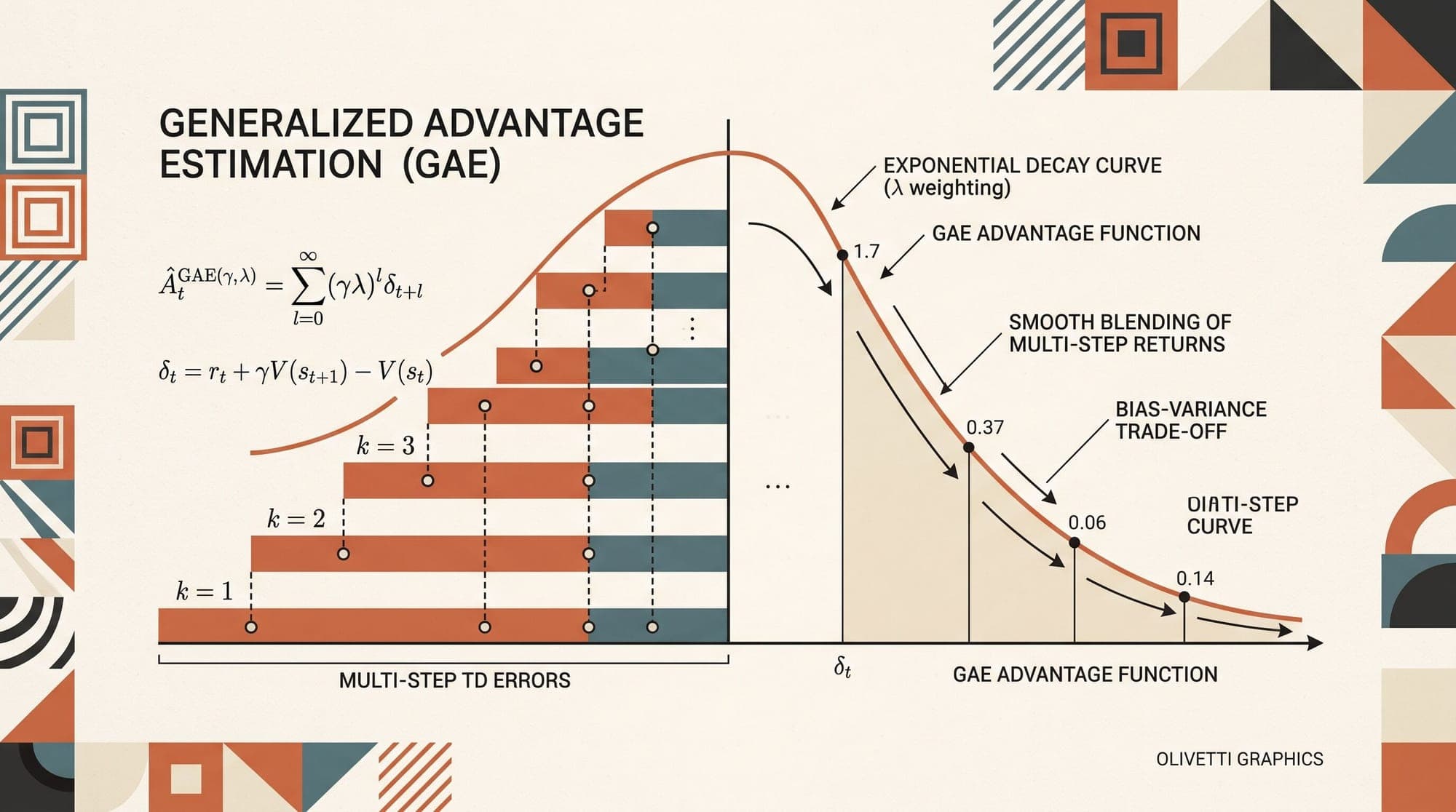
In their 2015 paper, Schulman et al. proposed defining the Generalized Advantage Estimator A_hat_t^GAE(gamma, lambda) as the exponentially weighted average of all k-step advantage estimators:

A_hat_t^GAE(gamma, lambda) = (1 - lambda) * sum_{k=1}^infinity lambda^(k-1) * A_hat_t^(k)

Expanding this geometric combination yields a direct sum of discounted TD residuals:

A_hat_t^GAE(gamma, lambda) = sum_{l=0}^infinity (gamma * lambda)^l * delta_{t+l}^V

This formulation mirrors the classical TD(lambda) algorithm introduced by Sutton for value estimation, but applies the exponential decay parameter lambda in [0, 1] specifically to advantage estimation for policy gradient updates.

Boundary Cases and the Role of Lambda

The parameter lambda acts as a continuous dial between bias and variance:

1. lambda = 0: GAE collapses to the 1-step TD residual A_hat_t^GAE(gamma, 0) = delta_t^V = r_t + gamma * V_phi(s_{t+1}) - V_phi(s_t). This minimizes variance by evaluating value function estimates at every subsequent step, but introduces maximum bias if V_phi is misspecified.
2. lambda = 1: GAE collapses to the empirical Monte Carlo return minus baseline A_hat_t^GAE(gamma, 1) = sum_{l=0}^infinity gamma^l * delta_{t+l}^V = sum_{l=0}^infinity gamma^l * r_{t+l} - V_phi(s_t). This eliminates baseline approximation bias from intermediate states, but exhibits maximum variance.
3. 0 < lambda < 1: Intermediate values compromise between bias and variance. The product gamma * lambda defines the effective decay rate of future temporal difference corrections.

Recursive computation makes GAE computationally efficient to calculate over finite rollouts of length T:

A_hat_t^GAE = delta_t^V + (gamma * lambda) * A_hat_{t+1}^GAE

Working backwards from timestep T-1 down to 0, GAE evaluates all advantage estimates in O(T) time with zero matrix operations.

Value Function Fitting and Advantage Normalization

In actor-critic architectures, the value network V_phi(s) is trained alongside the policy network pi_theta(a | s). GAE advantages provide both the policy gradient weights and the regression targets for updating V_phi.

The value function target R_hat_t is constructed by adding the estimated advantage back to the current value prediction:

R_hat_t = A_hat_t^GAE(gamma, lambda) + V_phi(s_t)

The value network parameters are optimized via mean squared error regression:

L(phi) = 1/|B| * sum_{t in B} (V_phi(s_t) - R_hat_t)^2

Before passing advantage estimates into policy gradient objectives such as TRPO or PPO, standard practice applies batch normalization:

A_norm_t = (A_hat_t - mean(A_hat)) / (std(A_hat) + eps)

Advantage normalization standardizes gradient scale across training iterations, preventing early reward scale variations from destabilizing learning rates.

Standard Empirical Hyperparameters

Across continuous control benchmarks (such as MuJoCo) and discrete environments, empirical studies by Schulman et al. established standard hyperparameter ranges:

• Discount factor: gamma in [0.99, 0.995]
• GAE decay parameter: lambda in [0.95, 0.98]

Setting lambda = 0.95 retains sufficient multi-step signal to mitigate value function errors while damping long-horizon trajectory noise. When applied to Proximal Policy Optimization (PPO), these default parameters became the de facto standard across deep reinforcement learning libraries.

GAE in LLM Alignment vs. Critic-Free Baselines

When reinforcement learning was adapted for large language models in InstructGPT (Ouyang et al., 2022) and subsequent RLHF pipelines, GAE served as the core advantage estimator.

In token-level autoregressive generation:

1. The state s_t consists of the prompt tokens and all generated tokens up to position t.
2. The action a_t is the generated token at position t.
3. Intermediate rewards r_t are zero for t < T, with a per-token KL divergence penalty against a reference policy pi_ref. The scalar reward model score is added at the final terminal token T.
4. A token-level critic network V_phi(s_t) estimates the expected final sequence reward from each token prefix.
5. GAE propagates the terminal outcome reward and per-token KL penalties backward through the sequence.

While effective, token-level GAE imposes heavy infrastructure demands on frontier model training. Running a separate value model of equivalent parameter size (for example, a 70-billion-parameter critic alongside a 70-billion-parameter actor) doubles VRAM allocation and requires synchronized distributed training passes. Furthermore, fitting token-level value networks on long reasoning trajectories can be noisy and prone to reward hacking.

To address these memory and credit assignment bottlenecks, recent reasoning model architectures, such as DeepSeekMath (Shao et al., 2024) and DeepSeek-R1 (DeepSeek-AI, 2025), introduced Group Relative Policy Optimization (GRPO). GRPO eliminates the critic network and GAE entirely. Instead, it samples a group of candidate outputs for each prompt, evaluates their trajectory-level rule-based or verifier rewards, and computes advantages by standardizing scores across the group:

A_i = (r_i - mean(r_group)) / (std(r_group) + eps)

While GRPO discards intermediate temporal credit assignment in favor of compute efficiency, Generalized Advantage Estimation remains the foundational reference framework for value-based actor-critic policy optimization in reinforcement learning.

Sources

• High-Dimensional Continuous Control Using Generalized Advantage Estimation (Schulman et al., 2015)
• Policy Gradient Methods for Reinforcement Learning with Function Approximation (Sutton et al., 1999)
• Trust Region Policy Optimization (Schulman et al., 2015)
• Proximal Policy Optimization Algorithms (Schulman et al., 2017)
• Training language models to follow instructions with human feedback (Ouyang et al., 2022)
• DeepSeekMath: Pushing the Limits of Mathematical Reasoning in Open Language Models (Shao et al., 2024)
• DeepSeek-R1: Incentivizing Reasoning Capability in LLMs via Reinforcement Learning (DeepSeek-AI, 2025)