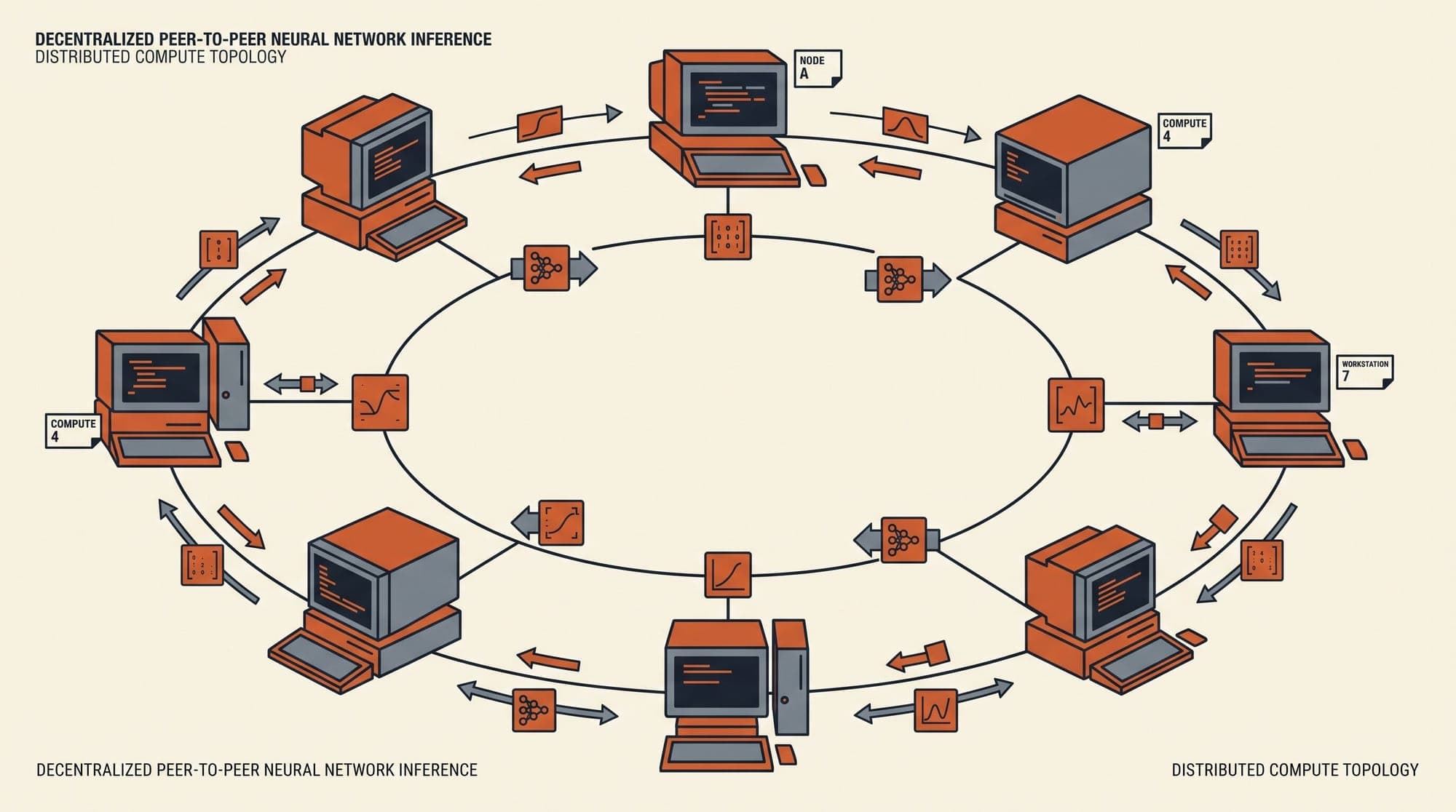
Decentralized and Peer-to-Peer LLM Inference in Production: Architecture, Ring Memory Partitioning, and Network Latency

Frontier open-weight models such as Llama 3.1 405B, DeepSeek-V3, and Command R+ have expanded model capabilities, but their parameter scales exceed the physical memory limits of individual consumer and edge workstations. Running a 405-billion parameter model in 16-bit precision requires over 810 GB of memory, and even 4-bit quantized variants require roughly 230 GB of contiguous VRAM or unified memory. While hyperscalers address this through high-density clusters unified by proprietary NVLink switches and ultra-low-latency InfiniBand fabrics, decentralized and peer-to-peer (P2P) inference runtimes take an alternative route: pooling consumer devices across local area networks (LAN) and wide area networks (WAN).

Frameworks such as Exo, Petals, and llama.cpp RPC implement decentralized inference across heterogeneous hardware. Understanding how these systems partition model layers, manage network serialization, and handle node churn reveals the trade-offs between local compute sovereignty and serving throughput.

Parallelism Strategies on Commodity Interconnects

The core challenge of distributed inference on consumer networks is the bandwidth-to-latency asymmetry between data-center fabrics and commodity interconnects. Data-center clusters rely on NVLink (providing up to 1.8 TB/s bidirectional bandwidth with sub-microsecond latency) or RoCEv2/InfiniBand (400 Gbps to 800 Gbps). In contrast, local clusters operate over Thunderbolt 4/5 (40 to 80 Gbps), 10 GbE, 1 GbE, or standard Wi-Fi, while public swarms operate over variable WAN connections (10 to 100 Mbps).

This network constraint dictates the choice of distributed execution strategy:

Tensor Parallelism Bottlenecks

Tensor Parallelism (TP) splits individual weight matrices (such as attention projection matrices $W_q, W_k, W_v, W_o$ and feed-forward matrices $W_{gate}, W_{up}, W_{down}$) across devices. In Megatron-style tensor parallelism, each transformer layer requires two All-Reduce collective communication steps: one after the multi-head attention block and one after the MLP block.

For an 80-layer architecture like Llama 3.1 70B, generating a single token requires 160 network synchronizations. On interconnects with millisecond-scale latency, the cumulative network wait time dominates computation, reducing generation speeds to fractions of a token per second. Consequently, tensor parallelism across separate physical machines is viable only over high-speed direct links, such as Thunderbolt RDMA using backends like Apple MLX Distributed (jaccl).

Pipeline Parallelism over Commodity Networks

Pipeline Parallelism (PP) partitions the model sequentially along its depth: device 0 executes layers 1 through $k_1$, device 1 executes layers $k_1+1$ through $k_2$, and device $N-1$ executes the final layers and computes token logits.

Under sequential pipeline parallelism, communication happens only at stage boundaries:

• Generation Phase (Decode): At each autoregressive step, device $i$ processes the single active token through its assigned layers and transmits only the resulting hidden state tensor $H \in \mathbb{R}^{1 \times d_{model}}$ to device $i+1$.
• Bandwidth Requirement: For a model with hidden dimension $d_{model} = 8192$ (such as Llama 3.1 70B) in FP16 precision, the activation tensor size per token is:

$$\text{Payload} = 1 \times 8192 \times 2 \text{ bytes} = 16,384 \text{ bytes (16 KB)}$$

• Network Cost: Transmitting 16 KB across a 1 Gbps Ethernet connection requires roughly 0.13 ms of wire time. Even factoring in TCP socket serialization and kernel context switches, transfer latency remains under 2 ms per boundary.

Because pipeline parallelism requires only $N-1$ sequential point-to-point transfers per token, it serves as the primary execution engine for decentralized P2P frameworks.

Ring Memory-Weighted Partitioning Architecture

In homogeneous data centers, pipeline stages are split evenly. In consumer and edge environments, however, clusters consist of heterogeneous nodes: for example, a Mac Studio with 192 GB unified memory, a MacBook Pro with 36 GB, and a Linux workstation with an RTX 4090 (24 GB VRAM).

To maximize aggregate throughput, modern decentralized engines like Exo implement Ring Memory-Weighted Partitioning.

Layer Allocation Mechanics

Let $N$ be the number of active nodes in the cluster, where each node $i$ reports available memory capacity $M_i$. The total available cluster memory is:

$$M_{total} = \sum_{i=1}^N M_i$$

For a model with $L$ total transformer layers, the contiguous layer partition $[S_i, E_i)$ assigned to node $i$ is calculated proportional to its memory contribution:

$$\text{Layer Count}_i = \text{round}\left(L \cdot \frac{M_i}{M_{total}}\right)$$

class RingMemoryWeightedPartitioning:
    def partition(self, nodes: list[Node], total_layers: int) -> list[Partition]:
        total_memory = sum(node.available_memory_bytes for node in nodes)
        partitions = []
        current_layer = 0
        
        for i, node in enumerate(nodes):
            if i == len(nodes) - 1:
                end_layer = total_layers
            else:
                weight = node.available_memory_bytes / total_memory
                allocated_layers = int(round(total_layers * weight))
                end_layer = min(current_layer + allocated_layers, total_layers)
                
            partitions.append(Partition(
                node_id=node.id,
                start_layer=current_layer,
                end_layer=end_layer,
                layer_count=end_layer - current_layer
            ))
            current_layer = end_layer
            
        return partitions

Ring Topology Execution Flow

In a ring topology, requests and activations flow along a directed cycle:

1. Prompt Ingestion: The client sends an inference request (HTTP/gRPC OpenAI-compatible API) to any node in the cluster. This node acts as the coordinator for the request lifecycle.
2. Sequential Forwarding: Node 0 embeds input tokens and computes forward activations for layers $[0, k_1)$. It serializes the intermediate activation tensor and streams it to Node 1.
3. Pipelined Evaluation: Each subsequent node executes its assigned block of layers against its local Key-Value (KV) cache.
4. Logit Computation and Sampling: The terminal node evaluates the final transformer block, applies the RMS normalization layer, projects activations via the language model head ($W_{unembed}$), and samples the next token ID.
5. Ring Feedback: The sampled token ID is sent back to Node 0 to trigger the subsequent autoregressive step, completing the ring.

By decoupling the coordinator role from a fixed centralized master, decentralized architectures eliminate single-point-of-failure bottlenecks.

Architecture Comparison: Exo vs. Petals vs. llama.cpp RPC

Different decentralized frameworks make distinct architectural trade-offs across discovery protocols, backend integration, network scale, and security boundaries.

1. Exo (Local and Hybrid Mesh Clusters)

• Target Environment: Local area networks, mixed Apple Silicon unified memory systems, and cross-platform GPUs (NVIDIA, AMD).
• Discovery Protocol: Zero-configuration UDP multicast and mDNS broadcast on local subnets, with support for Tailscale overlay networks.
• Inference Engines: Pluggable engine abstraction supporting Apple MLX (Metal acceleration) and Tinygrad (CUDA/ROCm/Metal JIT compilation).
• Partitioning Model: Dynamic ring memory-weighted pipeline partitioning and tensor sharding over Thunderbolt RDMA.
• Failure Recovery: Dynamic heartbeat monitoring; when a node drops, the remaining nodes trigger cluster re-benchmarking and recalculate layer boundaries.

2. Petals (Public Swarms and Internet-Scale P2P)

• Target Environment: Public wide-area networks with untrusted, volunteer-operated GPU servers.
• Discovery and Routing: Built on Hivemind and libp2p Kademlia Distributed Hash Tables (DHT). Nodes advertise hosted blocks (e.g., layers 16 to 32) in the DHT.
• Fault-Tolerant Routing: Clients dynamically construct an inference path through available peers based on measured ping latency and reported throughput. If a peer fails mid-generation, the client falls back to an alternative peer hosting the same layer block.
• Privacy Model: Implements selective activation compression (8-bit quantized activation forwarding) and experimental multi-party routing, though full prompt privacy on public swarms remains an open research challenge.

3. llama.cpp RPC (Client-Server Offloading)

• Target Environment: Dedicated local networks connecting secondary machines to a primary orchestrator.
• Architecture: Client-server remote procedure call model. A single primary instance of llama.cpp acts as the coordinator, dispatching backend compute operations (ggml backend) to remote RPC worker daemons over standard TCP sockets.
• Partitioning Model: Static layer and tensor distribution defined at launch via command-line arguments.
• Failure Recovery: Minimal fault tolerance; an unhandled socket drop terminates the inference process.

Memory Management and KV Cache Allocation

In distributed pipeline inference, memory consumption splits into two components: static parameter weights and dynamic KV cache state.

KV Cache Isolation

A major benefit of pipeline partitioning is that each node only maintains the KV cache for its assigned subset of layers:

$$\text{KV Cache Size per Token}_i = 2 \times (\text{End Layer}_i - \text{Start Layer}_i) \times n_{kv\_heads} \times d_{head} \times \text{dtype\_bytes}$$

For a model with Grouped-Query Attention (GQA), such as Llama 3.1 70B ($n_{kv\_heads} = 8, d_{head} = 128$), each assigned layer consumes 4 KB per token in 16-bit precision. A node hosting 20 layers requires only 80 KB per token of sequence context, distributing the context memory burden proportionally across the cluster.

Prefill vs. Decode Activation Dynamics

Distributed pipelines exhibit different bottleneck profiles across inference phases:

• Prefill Phase (Prompt Processing): The prompt tensor $X \in \mathbb{R}^{B \times S \times d_{model}}$ is compute-dense but produces large activation payloads between pipeline stages. For a prompt length $S = 4096$, transferring activations between nodes requires transmitting:

$$\text{Payload}_{prefill} = 4096 \times 8192 \times 2 \text{ bytes} = 67.1 \text{ MB}$$ Over a 1 GbE link, transmitting 67.1 MB takes ~540 ms of pure network transfer time. Consequently, prompt prefilling on slow interconnects suffers noticeable Time-to-First-Token (TTFT) degradation.

• Decode Phase (Token Generation): Generation is memory-bandwidth bound and transmits only 16 KB per step. Network transmission takes <2 ms, allowing generation speeds to match the memory bandwidth limits of the slowest node in the pipeline.

Production Trade-Offs and Failure Boundaries

Decentralized and P2P inference offers distinct advantages for specific deployment profiles while introducing clear architectural constraints:

Advantages

1. Hardware Capitalization: Eliminates the necessity of acquiring enterprise H100/B200 clusters to evaluate or fine-tune 70B to 405B parameter models.
2. Unified Memory Utilization: Exploits high-capacity, lower-cost unified memory architectures (such as Apple Silicon M-series chips with up to 192 GB unified RAM) that provide high local memory bandwidth without data-center power infrastructure.
3. Zero Configuration Setup: Local P2P discovery automates cluster assembly without complex Kubernetes orchestration or manual host configuration.

Operational Challenges

1. Interconnect Latency Floor: Generation throughput is bounded by the sum of per-node computation times plus $(N-1) \times \text{network round-trip time}$. Over standard Wi-Fi or residential broadband, total latency caps decoding at 2 to 6 tokens per second.
2. Pipeline Bubble Inefficiency: In pure sequential pipeline parallelism with batch size 1, only one node computes at any given micro-instant while other nodes remain idle. Achieving high GPU utilization requires micro-batching and 1F1B (One Forward, One Backward) scheduling, which increases memory overhead and scheduling complexity.
3. KV Cache Loss on Disconnection: If a node disconnects during generation, its locally held KV cache state is lost. Recovering requires electing a new pipeline configuration and re-evaluating the prompt from scratch (or re-hydrating the KV cache), introducing substantial latency spikes.

Sources

• Petals: Distributed Inference and Fine-tuning of Large Language Models Over the Internet (NeurIPS 2023)
• Exo GitHub Repository and Architecture Specification
• Apple MLX Framework: Distributed Multi-Device Operations
• Hivemind: Decentralized Deep Learning Framework
• llama.cpp: Remote Procedure Call (RPC) Backend Documentation