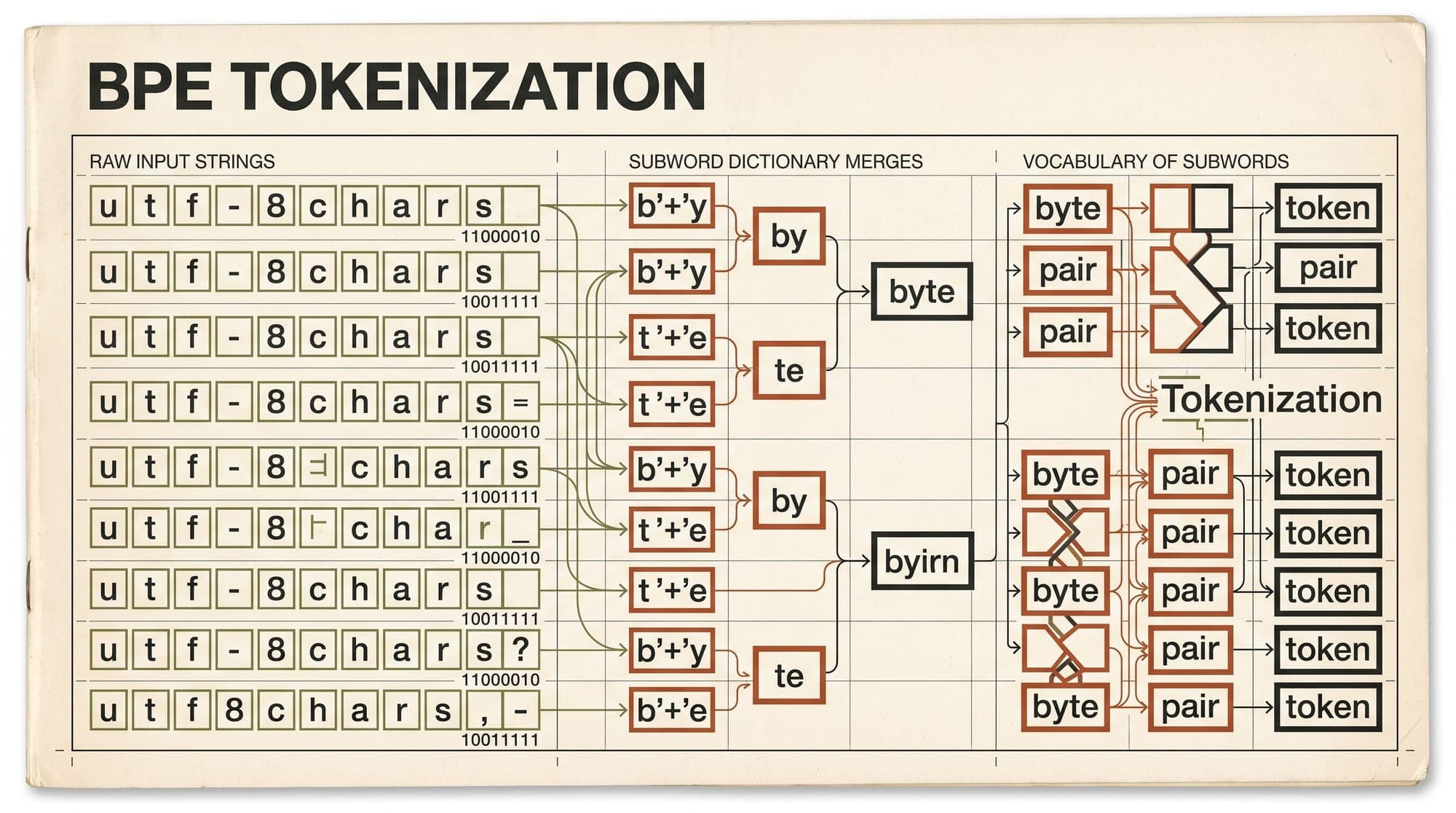
Byte-Pair Encoding (BPE): Mathematical Foundations, Merge Table Dynamics, Byte-Level Fallbacks, and Vocabulary Compression in Large Language Models

Every large language model operates on discrete numerical tokens rather than raw text strings. The translation layer between human language and model tensor activations is governed by subword tokenization algorithms. Among these, Byte-Pair Encoding (BPE) has emerged as the dominant standard across modern foundation models, including OpenAI's GPT-4, Meta's Llama 3, and Alibaba's Qwen 2.5.

Originally developed by Philip Gage (1994) for data compression, BPE was adapted for natural language processing by Sennrich et al. (2016) to resolve the out-of-vocabulary (OOV) challenge in neural machine translation. It was subsequently extended to raw UTF-8 byte streams by Radford et al. (2019) in GPT-2.

This article examines the mathematical formulation of BPE, its merge dynamics, byte-level fallback mechanics, comparative trade-offs against WordPiece and Unigram models, vocabulary scaling economics, and known structural pathologies.

1. The Tokenization Trade-Off: Sequence Length vs. Vocabulary Size

Autoregressive language models process input text as a sequence of discrete embedding vectors. Designing the discrete vocabulary $\mathcal{V}$ introduces a fundamental trade-off between sequence length $T$ and vocabulary size $|\mathcal{V}|$ :

Character-Level Representation ( $|\mathcal{V}| \approx 256$ to $10^3$ ):

Advantage: Minimal vocabulary size; zero out-of-vocabulary rate.
Disadvantage: High sequence length $T$ . Because transformer self-attention exhibits $O(T^2)$ computational complexity and linear key-value (KV) cache memory scaling ( $2 \cdot L \cdot H \cdot D \cdot T$ ), character-level tokenization imposes severe latency and memory overhead.

Word-Level Representation ( $|\mathcal{V}| \approx 10^6$ to $10^7$ ):

Advantage: Short sequence lengths $T$ .
Disadvantage: Exponential vocabulary explosion; inability to process unseen words (leading to out-of-vocabulary tokens, denoted as <unk>); massive embedding and unembedding weight matrices ( $|\mathcal{V}| \times d_{\text{model}}$ ) that dominate GPU memory and bandwidth.

Subword Representation ( $|\mathcal{V}| \approx 3 \times 10^4$ to $2.5 \times 10^5$ ):

Mechanism: Frequent full words remain single tokens, while rare words are decomposed into morphological subwords or individual characters/bytes.
Result: Optimizes the Pareto frontier between sequence length and vocabulary memory footprint.

2. Mathematical Formulation and Algorithm

BPE is a data-driven, bottom-up statistical compression algorithm that iteratively merges the most frequent co-occurring pairs of adjacent symbols.

Training Phase (Vocabulary and Merge Table Construction)

Let $\mathcal{D} = \{w_1, w_2, \dots, w_N\}$ be a tokenization training corpus represented as a sequence of words with corresponding frequencies $\{f(w_n)\}_{n=1}^N$ .

Initialization:

Define the initial base vocabulary $\mathcal{V}_0$ as the set of all unique individual characters (or UTF-8 bytes) present in $\mathcal{D}$ : $\mathcal{V}_0 = \text{UniqueSymbols}(\mathcal{D})$ Each word $w \in \mathcal{D}$ is initialized as a tuple of base symbols: $w = (c_1, c_2, \dots, c_m)$ .

Iterative Pair Extraction and Merging:

For each iteration $k = 1, 2, \dots, K$ , where $K = |\mathcal{V}_{\text{target}}| - |\mathcal{V}_0|$ :

Compute the co-occurrence frequency of every adjacent symbol pair $(c_i, c_j)$ across the segmented corpus:

$f(c_i, c_j) = \sum_{w \in \mathcal{D}} f(w) \cdot \text{count}_{(c_i, c_j)}(w)$

Identify the most frequent pair:

$(c_i^<em>, c_j^</em>) = \arg\max_{(c_i, c_j)} f(c_i, c_j)$

Form the new merged subword symbol:

$c_{\text{new}} = c_i^* \circ c_j^*$

Update the vocabulary:

$\mathcal{V}_k = \mathcal{V}_{k-1} \cup \{c_{\text{new}}\}$

Record the merge rule with rank $k$ :

$\mathcal{M}(c_i^<em>, c_j^</em>) = k$

Replace all adjacent occurrences of $(c_i^, c_j^)$ with $c_{\text{new}}$ across the entire corpus $\mathcal{D}$ .

Termination:

The loop terminates when $|\mathcal{V}_k| = |\mathcal{V}_{\text{target}}|$ or when the maximum pair frequency falls below a predefined threshold $\tau$ .

Corpus: "low", "lower", "newest", "widest"

Step 0: Initial symbols: {l, o, w, e, r, n, s, t, i, d}
Segmented:
  l o w </w>       (count: 5)
  l o w e r </w>   (count: 2)
  n e w e s t </w> (count: 6)
  w i d e s t </w> (count: 3)

Iteration 1: Most frequent pair = ('e', 's') [freq = 9]
Merge: 'es' -> Add 'es' to Vocab
Segmented: ... n e w es t </w>, w i d es t </w>

Iteration 2: Most frequent pair = ('es', 't') [freq = 9]
Merge: 'est' -> Add 'est' to Vocab
Segmented: ... n e w est </w>, w i d est </w>

Iteration 3: Most frequent pair = ('l', 'o') [freq = 7]
Merge: 'lo' -> Add 'lo' to Vocab
...

Inference Phase (Deterministic Encoding)

Given a raw input string, the encoder splits the text into initial base symbols and greedily applies the learned merge table $\mathcal{M}$ according to merge priority ranks:

Segment text into base tokens: $S = [c_1, c_2, \dots, c_m]$ .
Identify all candidate pairs $(c_j, c_{j+1})$ in $S$ that exist in $\mathcal{M}$ .
Select the candidate pair with the lowest rank index (highest training frequency):

$(c_j, c_{j+1})^* = \arg\min_{(c_j, c_{j+1}) \in S} \mathcal{M}(c_j, c_{j+1})$

Merge $(c_j, c_{j+1})$ into $c_{\text{new}}$ and update sequence $S$ .
Repeat steps 2 to 4 until no adjacent pair in $S$ exists in $\mathcal{M}$ .

3. Byte-Level Byte-Pair Encoding (BBPE) and Regex Pre-Tokenization

Early BPE implementations operated on Unicode characters. In multilingual corpora containing thousands of distinct Unicode code points (such as CJK characters, Cyrillic, and emojis), character-level base vocabularies $\mathcal{V}_0$ exceeded tens of thousands of symbols before any merge operations began, frequently producing <unk> tokens for rare characters.

Byte-Level Base Vocabulary

To resolve this limitation, Radford et al. (2019) introduced Byte-Level BPE in GPT-2.

Base Alphabet: Initialized with exactly 256 byte values ( $0\text{x}00$ through $0\text{xFF}$ ), representing all possible single-byte values in UTF-8 encoding.
Out-of-Vocabulary Guarantee: Because any arbitrary string can be serialized into a sequence of UTF-8 bytes, the out-of-vocabulary rate is strictly zero. The model never emits an <unk> token.
Byte Mapping: To ensure compatibility with standard string-processing tokenizers without control character corruption, raw byte values are mapped bijectively to printable Unicode characters.

Pre-Tokenization Splitting Rules

Naive byte-level BPE can merge across punctuation, whitespace, and numerical boundaries, leading to sub-optimal tokens such as "?the", "dog.", or mixed alphanumeric sequences.

To prevent this cross-boundary pollution, tokenizers apply regular expression pre-tokenization prior to BPE merging. The regex splits the input string into isolated chunks, and BPE merges are constrained to operate strictly within each chunk.

For example, the pre-tokenization regex utilized in Meta's Llama 3 is structured as follows:

# Llama 3 / tiktoken pre-tokenization pattern
r"""(?i:'s|'t|'re|'ve|'m|'ll|'d)|[^\r\n\p{L}\p{N}]?\p{L}+|\p{N}{1,3}| ?[^\s\p{L}\p{N}]+[\r\n]*|\s*[\r\n]+|\s+(?!\S)|\s+"""

This pattern enforces distinct operational rules:

Contractions: Separates English contractions ('s, 't, 're) into dedicated segments.
Alphabetic Chunks: Keeps letter sequences distinct from numbers and punctuation.
Numeric Splitting: Limits digit groupings (\p{N}{1,3}), preventing arbitrary multi-digit concatenation.
Whitespace and Newlines: Segments consecutive spaces and line breaks independently.

4. Algorithmic Comparison: BPE vs. WordPiece vs. Unigram

Modern language models rely on three distinct subword tokenization paradigms:

1. Byte-Pair Encoding (BPE)

Primary Reference: Sennrich et al. (2016)
Construction Direction: Bottom-up (Iterative merging)
Optimization Objective: Raw co-occurrence frequency $\max f(u, v)$
Inference Mechanism: Deterministic merge rank replay
Stochastic Regularization: BPE-Dropout (stochastically skipping merge steps during training)
Notable Deployments: GPT-4, Llama 3, Qwen 2.5, Mistral

2. WordPiece

Primary Reference: Schuster & Nakajima (2012) and Wu et al. (2016)
Construction Direction: Bottom-up (Iterative merging)
Optimization Objective: Corpus likelihood / mutual information ratio:

$\text{Score}(u, v) = \frac{\text{count}(uv)}{\text{count}(u) \times \text{count}(v)}$ This normalizes pair counts by their marginal token frequencies, prioritizing pairs whose components rarely occur independently over pairs composed of ubiquitous individual characters.

Inference Mechanism: Greedy longest-prefix matching
Notable Deployments: BERT, DistilBERT, Electra

3. Unigram Language Model

Primary Reference: Kudo (2018)
Construction Direction: Top-down (Iterative pruning from an over-complete seed vocabulary)
Optimization Objective: Marginal corpus log-likelihood under unigram assumption:

$\mathcal{L} = \sum_{i=1}^N \log \left( \sum_{x \in S(w_i)} P(x) \right), \quad P(x) = \prod_{t \in x} p(t)$ where $S(w_i)$ represents all valid token segmentations of word $w_i$ . Tokens with the lowest loss impact upon removal are pruned in batches.

Inference Mechanism: Dynamic programming via the Viterbi algorithm
Stochastic Regularization: Native Subword Regularization (sampling segmentations from the posterior distribution $P(x|w)$ during training)
Notable Deployments: T5, ALBERT, Gemma (SentencePiece Unigram)

5. Vocabulary Scaling and Serving Economics

The scale of foundation model vocabularies has expanded substantially across model generations:

GPT-2 (2019): 50,257 tokens
LLaMA 1 & 2 (2023): 32,000 tokens
Llama 3 (2024): 128,256 tokens (Meta AI, 2024)
Qwen 2.5 (2024): 151,936 tokens (Qwen Team, 2024)
Gemma 2 (2024): 256,000 tokens

Vocabulary Size Evolution:
GPT-2 (2019):    [50,257]
LLaMA 2 (2023):  [32,000]
Llama 3 (2024):  [128,256]
Qwen 2.5 (2024): [151,936]
Gemma 2 (2024):  [256,000]

Compression Ratio vs. Sequence Length

Expanding the vocabulary size increases token compression efficiency. For example, upgrading from LLaMA 2's 32k vocabulary to Llama 3's 128k vocabulary yielded an average ~15% reduction in total token count across multilingual and code benchmarks:

$\text{Compression Ratio} = \frac{\text{Bytes of Raw Text}}{\text{Number of Emitted Tokens}}$

Higher compression ratios provide direct operational benefits in serving:

Autoregressive Decoding Speed: Generating a fixed semantic response requires fewer total decoding steps ( $T_{\text{gen}}$ ), speeding up generation throughput.
KV Cache Footprint: Total KV cache memory per request scales linearly with sequence length $T$ . A 15% reduction in tokens yields a 15% reduction in active KV cache memory allocation ( $2 \cdot L \cdot H \cdot D \cdot T$ ).
Prefill Latency (TTFT): Time-to-first-token decreases because fewer prompt tokens enter initial matrix multiplications.

Hardware Memory and Compute Trade-Offs

Increasing vocabulary size introduces concrete hardware costs in the input embedding and output unembedding (lm_head) layers:

$\text{Parameter Overhead} = 2 \times |\mathcal{V}| \times d_{\text{model}}$

For a model with hidden dimension $d_{\text{model}} = 8192$ and vocabulary size $|\mathcal{V}| = 128,256$ in BF16 precision (2 bytes per parameter):

The input embedding table requires $128,256 \times 8192 \times 2 \approx 2.10\text{ GB}$ of VRAM.
The unembedding matrix requires another $2.10\text{ GB}$ of VRAM.
Computing output logits requires an $[B, d_{\text{model}}] \times [d_{\text{model}}, |\mathcal{V}|]$ matrix multiplication followed by a softmax reduction over 128,256 elements per generation step, increasing memory bandwidth demands during decoding.

6. Structural Pathologies and Failure Modes

Despite its universal deployment, BPE exhibits several known algorithmic and linguistic failure modes:

1. The Multilingual "Token Tax"

BPE merge frequencies are directly determined by the composition of the pre-training corpus. In predominantly English corpora, English text achieves high compression (~3.5 to 4.5 characters per token).

In contrast, low-resource scripts (such as Devanagari, Telugu, Thai, or Arabic) under-represented in the corpus fail to accumulate sufficient merge counts. Consequently, words in these languages are segmented into single-byte or two-byte tokens (yielding 1 to 1.5 characters per token).

This disparity creates a systemic "token tax": non-Latin languages consume 2x to 5x more tokens to convey equivalent semantic content, inflating API inference costs and effectively compressing the model's usable context window. Modern architectures (such as Qwen 2.5 and Llama 3) mitigate this by explicitly upsampling multilingual data during tokenizer training and scaling vocabulary size beyond 128k.

2. Glitch Tokens and Polysemantic Embeddings

When web corpora are scraped, anomalies such as repeated automated log strings, code formatting artifacts, or specific forum usernames (e.g. SolidGoldMagikarp, StreamerBot) appear with high frequency in tokenizer training sets, earning dedicated tokens in the vocabulary table.

However, if these strings are subsequently stripped from pre-training datasets by decontamination or filtering pipelines, their corresponding embedding vectors receive near-zero gradient updates during model training. In production, prompting the model with these "glitch tokens" causes anomalous distance metrics in embedding space, triggering severe hallucinations, repetitive degeneration, or safety jailbreaks.

3. Arithmetic and Numerical Token Fragmentation

Unless constrained by specialized regex pre-tokenizers, BPE merges multi-digit numbers based on corpus frequency. For instance, common numbers like "1984" or "2024" might merge into single tokens, while "1985" is split into "198" and "5", and "2025" into "20" and "25".

This inconsistent tokenization impairs arithmetic reasoning. The neural network cannot execute uniform column-wise arithmetic algorithms when numbers are inconsistently partitioned into variable-length digit chunks. Modern tokenizers enforce explicit single-digit or fixed-digit regex splitting (e.g., \p{N} or \p{N}{1,3}) to preserve structural regularity in mathematical contexts.