Adaptive Optimizers in Large Language Model Pre-Training: How AdamW, Adafactor, and Lion Scale Gradient Updates Across Billions of Parameters

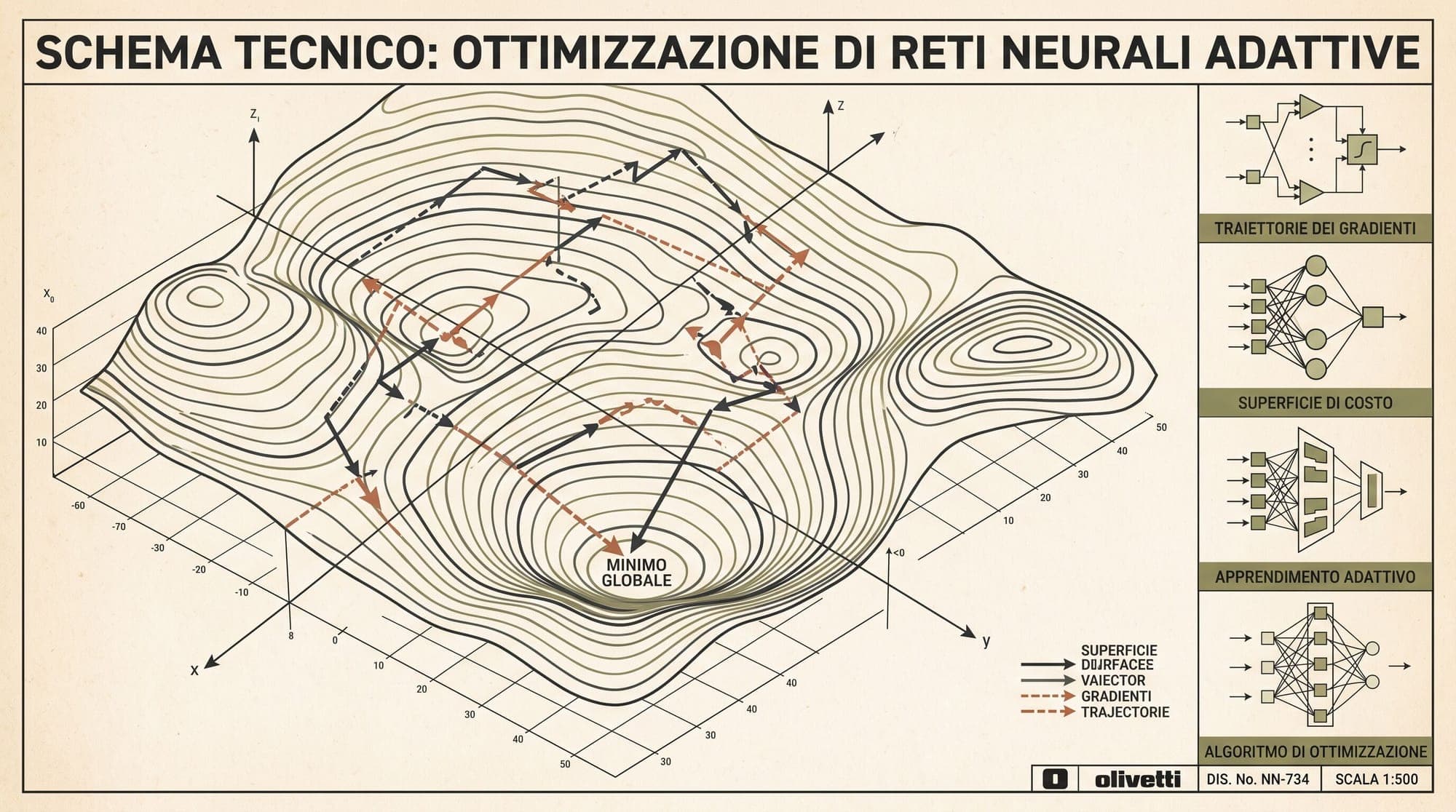
Large language model pre-training requires optimizing billions of parameters over trillions of tokens across distributed GPU clusters. Standard stochastic gradient descent (SGD) fails in this regime because Transformer loss landscapes are severely ill-conditioned, with gradient magnitudes differing by orders of magnitude across layers and token positions.

To train deep autoregressive models stably, modern deep learning relies on adaptive optimizers that scale update steps coordinate-by-coordinate using running gradient statistics. However, tracking historical moments introduces a steep memory and compute tax. Across large model architectures, optimizer states often consume more High Bandwidth Memory (HBM) than the model weights themselves.

Understanding how optimizers balance convergence speed, numerical stability, and memory overhead is central to scaling modern foundation models.

The Ill-Conditioned Landscape of Transformer Gradients

Stochastic gradient descent updates parameters along the negative gradient vector:

$$w_{t+1} = w_t - \eta \nabla \mathcal{L}(w_t)$$

SGD assumes that a single global learning rate $\eta$ is appropriate for all dimensions in parameter space. In multi-layer Transformer architectures, this assumption breaks down due to three structural factors:

1. Extreme Curvature Anisotropy: The loss landscape exhibits an ill-conditioned Hessian matrix $\nabla^2 \mathcal{L}(w)$, where the condition number (the ratio of the largest to smallest eigenvalue, $\kappa = \lambda_{\max} / \lambda_{\min}$) frequently exceeds $10^6$. Updates with a fixed learning rate oscillate along high-curvature ravines while making negligible progress along flat directions.
2. Sparse vs. Dense Activation Dynamics: Embedding layers and unembedding projection heads receive sparse updates because only tokens present in a given batch generate non-zero gradients. In contrast, self-attention projection weights (Query, Key, Value, Output) and feed-forward gating layers receive dense activations on every token pass.
3. Heavy-Tailed Gradient Distributions: Gradients in deep attention layers frequently experience sudden magnitude spikes caused by softmax score concentrations and layer normalization interactions.

Coordinate-wise adaptive optimizers solve this by tracking past gradient history per parameter, effectively approximating a diagonal pre-conditioner that normalizes the step size across every dimension.

The Anatomy of Adam and the Weight Decay Fix

The foundation of modern LLM optimization is Adam (Adaptive Moment Estimation), introduced by Diederik Kingma and Jimmy Ba in 2014 (Kingma & Ba, 2014). Adam tracks two moving averages for every parameter:

• First Moment ($m_t$): The exponentially smoothed mean of past gradients (momentum), which dampens high-frequency oscillations.
• Second Raw Moment ($v_t$): The exponentially smoothed uncentered variance of past gradients, which estimates the squared scale of each coordinate.

$$\begin{aligned} m_t &= \beta_1 m_{t-1} + (1 - \beta_1) g_t \\ v_t &= \beta_2 v_{t-1} + (1 - \beta_2) g_t^2 \end{aligned}$$

Because $m_t$ and $v_t$ are initialized to zero vectors, they are biased toward zero in the initial training steps. Adam corrects this using step-dependent bias correction factors:

$$\hat{m}_t = \frac{m_t}{1 - \beta_1^t}, \quad \hat{v}_t = \frac{v_t}{1 - \beta_2^t}$$

The parameter update is then computed coordinate-wise:

$$w_{t+1} = w_t - \frac{\eta}{\sqrt{\hat{v}_t} + \epsilon} \hat{m}_t$$

Here, $\epsilon$ (typically $10^{-8}$ to $10^{-15}$) prevents division by zero, and $\beta_1, \beta_2$ are decay coefficients (conventionally set to $0.9$ and $0.95$ or $0.999$).

Standard Adam vs. Decoupled AdamW Parameter Updates

[Adam with L2 Regularization]
  g_t' = g_t + λ * w_t
  v_t  = β2 * v_{t-1} + (1 - β2) * (g_t')^2
  w_{t+1} = w_t - η * m_t / (sqrt(v_t) + ε)
  (Problem: Parameters with large gradient scale receive LESS weight decay)

[AdamW with Decoupled Weight Decay]
  v_t  = β2 * v_{t-1} + (1 - β2) * (g_t)^2
  w_{t+1} = w_t - η * λ * w_t - η * m_t / (sqrt(v_t) + ε)
  (Result: Uniform weight shrinkage rate η*λ across all coordinates)

Why L2 Regularization Broke Adam

In standard SGD, adding an $L_2$ penalty $\frac{1}{2}\lambda \|w\|_2^2$ to the loss function is mathematically identical to weight decay:

$$\nabla \left( \mathcal{L}(w) + \frac{1}{2}\lambda \|w\|_2^2 \right) = \nabla \mathcal{L}(w) + \lambda w$$

$$w_{t+1} = w_t - \eta (\nabla \mathcal{L}(w_t) + \lambda w_t) = (1 - \eta \lambda) w_t - \eta \nabla \mathcal{L}(w_t)$$

In adaptive gradient methods, this equivalence fails. When $L_2$ regularization is incorporated by modifying the gradient input ($g_t' = g_t + \lambda w_t$), the regularization term is divided by $\sqrt{\hat{v}_t} + \epsilon$:

$$w_{t+1} = w_t - \frac{\eta}{\sqrt{\hat{v}_t} + \epsilon} \left( \hat{m}_t(g_t) + \lambda w_t \right)$$

As demonstrated by Ilya Loshchilov and Frank Hutter in 2017 (Loshchilov & Hutter, 2017), this causes severe distortions:

• Parameters with frequent, large gradients (high $v_t$) experience suppressed weight decay because the penalty is scaled down by $\frac{1}{\sqrt{v_t}}$.
• Parameters with small or sparse gradients (low $v_t$) experience disproportionately large weight decay penalties.

The AdamW Formulation

AdamW resolves this distortion by decoupling weight decay from the gradient update step. The decay is applied directly to the parameter vector before or after the adaptive step:

$$w_{t+1} = w_t - \eta_t \lambda w_t - \eta_t \frac{\hat{m}_t}{\sqrt{\hat{v}_t} + \epsilon}$$

Decoupled weight decay ensures that every parameter shrinks at a uniform rate proportional to $\eta_t \lambda$, regardless of gradient variance. This separation restored the generalization performance of adaptive methods to match or exceed tuned SGD on complex benchmarks, establishing AdamW as the industry standard for LLM pre-training.

The Memory Tax of Optimizer States

In 16-bit mixed-precision pre-training (using BF16 or FP16 for forward and backward passes), model parameters and gradients each consume 2 bytes per parameter.

However, accumulating gradient moments directly in 16-bit formats leads to severe underflow, gradient stall, and numerical divergence. Consequently, standard implementations maintain optimizer states in full 32-bit floating point (FP32):

| Component | Precision | Bytes per Parameter | | :--- | :--- | :--- | | Model Weights | BF16 / FP16 | 2 bytes | | Gradients | BF16 / FP16 | 2 bytes | | Master Weights (FP32 copy) | FP32 | 4 bytes | | First Moment Buffer ($m_t$) | FP32 | 4 bytes | | Second Moment Buffer ($v_t$) | FP32 | 4 bytes | | Total Memory per Parameter | - | 16 bytes |

Memory Allocation per Parameter in Standard Mixed-Precision Training (16 Bytes Total)

┌──────────────┬──────────────┬─────────────────────────────┬─────────────────────────────┬─────────────────────────────┐
│ Weights      │ Gradients    │ Master Weights (FP32)       │ First Moment m_t (FP32)     │ Second Moment v_t (FP32)    │
│ (BF16)       │ (BF16)       │                             │                             │                             │
│ 2 Bytes      │ 2 Bytes      │ 4 Bytes                     │ 4 Bytes                     │ 4 Bytes                     │
└──────────────┴──────────────┴─────────────────────────────┴─────────────────────────────┴─────────────────────────────┘
                              └─────────────────────────────────────────────────────────────────────────────────────────┘
                                                       Optimizer State: 12 Bytes (75% of static memory)

For a 70-billion-parameter model:

• Model weights: 140 GB
• Gradients: 140 GB
• Optimizer states: 840 GB (FP32 master weights + $m_t$ + $v_t$)
• Total static memory footprint: 1.12 TB

Even when using distributed sharding techniques like ZeRO-1 or FSDP (which shard the 12 bytes of optimizer state across GPUs), optimizer state memory remains the primary constraint dictating cluster sizing and per-device batch limits.

Sublinear Memory via Factorization: Adafactor

To break the $O(N)$ memory scaling of second-moment tracking, Noam Shazeer and Mitchell Stern introduced Adafactor at ICML 2018 (Shazeer & Stern, 2018).

Low-Rank Matrix Decomposition

In a Transformer, the majority of parameters reside in 2D weight matrices $W \in \mathbb{R}^{r \times c}$ (e.g., attention projection matrices and MLP layers).

Instead of maintaining a full $r \times c$ matrix of second moments $V \in \mathbb{R}^{r \times c}$, Adafactor decomposes $V$ into row-wise and column-wise exponential moving averages:

$$\begin{aligned} R_t &= \beta_{2,t} R_{t-1} + (1 - \beta_{2,t}) \left( G_t^2 \mathbf{1}_c \right) \in \mathbb{R}^{r \times 1} \\ C_t &= \beta_{2,t} C_{t-1} + (1 - \beta_{2,t}) \left( \mathbf{1}_r^T G_t^2 \right) \in \mathbb{R}^{1 \times c} \end{aligned}$$

Here, $\mathbf{1}_c$ and $\mathbf{1}_r$ are all-ones vectors of dimension $c$ and $r$. At update time, Adafactor reconstructs an estimate of the full second-moment matrix $\hat{V}_t$ by minimizing the generalized Kullback-Leibler divergence (I-divergence):

$$\hat{V}_{t,ij} = \frac{R_{t,i} C_{t,j}}{\sum_{k=1}^r R_{t,k}}$$

Adafactor 2D Matrix Factorization

Full Second-Moment Matrix V (r x c)          Factorized Representation
┌───────────────────────────────────┐        Row Sums R (r x 1)     Column Sums C (1 x c)
│  v_11   v_12   ...   v_1c         │        ┌───────┐             ┌─────────────────────┐
│  v_21   v_22   ...   v_2c         │   =>   │  R_1  │      x      │ C_1   C_2  ...  C_c │
│  ...    ...    ...   ...          │        │  R_2  │             └─────────────────────┘
│  v_r1   v_r2   ...   v_rc         │        │  ...  │
└───────────────────────────────────┘        │  R_r  │
                                             └───────┘
  Memory: O(r * c)                             Memory: O(r + c)
  Example: 8192 x 8192 = 67.1M floats          Example: 8192 + 8192 = 16.38K floats
  (268.4 MB in FP32)                           (65.5 KB in FP32, a 99.97% reduction)

This reduces the memory requirement for the second moment from $O(rc)$ to $O(r + c)$. For an $8192 \times 8192$ weight matrix:

• Full matrix storage ($r \times c$): $67,108,864$ floats (268.4 MB in FP32).
• Factorized storage ($r + c$): $16,384$ floats (65.5 KB in FP32), representing a 99.97% reduction.

Dynamic Decay and Momentum Removal

Adafactor incorporates two additional architectural design choices:

1. Non-Constant Second-Moment Decay ($\beta_2$ Schedule): Adafactor replaces constant $\beta_2$ with a dynamic schedule:

$$\beta_{2,t} = 1 - t^{-\hat{\beta}_2}, \quad \text{where } \hat{\beta}_2 \in (0, 1] \text{ (typically } 0.8\text{)}$$ This places higher weight on recent gradients early in training and gradually stabilizes as steps accumulate.

1. Optional Momentum-Free Updates: To maximize memory savings, Adafactor can operate without maintaining a first-moment buffer ($m_t$), using gradient clipping via root-mean-square (RMS) normalization:

$$U_t = \frac{G_t}{\sqrt{\hat{V}_t}}, \quad \hat{U}_t = \frac{U_t}{\max\left(1, \frac{\text{RMS}(U_t)}{d}\right)}$$ Running momentum-free reduces optimizer state memory to less than 1 byte per parameter, enabling the training of models like T5 (Raffel et al., 2020) and PaLM (Chowdhery et al., 2022) under severe HBM constraints.

Lion: Symbolic Discovery and Uniform Step Magnitudes

In 2023, Xiangning Chen, Chen Liang, Da Huang, and collaborators at Google Brain and UCLA used symbolic program search over mathematical operations to discover Lion (evoLved Sign Momentum, Chen et al., 2023).

The Lion Algorithm

Lion discards second-moment tracking entirely and operates using only a single momentum buffer $m_t$. The update rule is defined by two separate interpolation operations:

$$\begin{aligned} c_t &= \text{sign}\left( \beta_1 m_{t-1} + (1 - \beta_1) g_t \right) \\ w_{t+1} &= w_t - \eta_t c_t - \eta_t \lambda w_t \\ m_t &= \beta_2 m_{t-1} + (1 - \beta_2) g_t \end{aligned}$$

Standard default parameters are $\beta_1 = 0.9$, $\beta_2 = 0.99$.

Lion Update Lifecycle

Gradient g_t ──────┐
                   ▼
Momentum m_{t-1} ──► Interpolate (β1=0.9) ──► sign(·) ──► Direction c_t ──► Update: w_{t+1} = w_t - η*c_t - η*λ*w_t
                   │
                   ▼
              Interpolate (β2=0.99) ──► Stored Momentum m_t

Key Differences from AdamW

1. Two Separate $\beta$ Splittings: Lion decouples the momentum used for computing the update direction ($c_t$, weighted by $\beta_1$) from the momentum preserved in state ($m_t$, updated with $\beta_2$). Because $\beta_1 < \beta_2$, Lion incorporates more of the instantaneous gradient into the directional step while maintaining a smoother history in memory.
2. The Sign Operator: Unlike AdamW, which scales steps inversely with $\sqrt{v_t}$, Lion computes updates using $\text{sign}(\cdot)$. Consequently, every coordinate moves by exactly $\pm \eta_t$ (prior to weight decay). This makes update magnitudes completely invariant to gradient scales across layers.
3. Implicit Regularization: The binary $\pm 1$ quantization introduces stochasticity into update directions, acting as a natural regularizer that enhances generalization on out-of-distribution benchmarks.
4. 50% State Memory Reduction: Because Lion only tracks $m_t$ (and no $v_t$), its optimizer state requires 4 bytes per parameter in FP32, compared to AdamW's 8 bytes.

Operational Constraints

Because every coordinate moves by $\pm \eta_t$, Lion's update norm is $\sqrt{d} \cdot \eta_t$ for a $d$-dimensional parameter tensor, whereas AdamW's update norm is bounded by the variance ratio. To prevent destabilization:

• Lion requires a learning rate roughly $3\times$ to $10\times$ smaller than AdamW (e.g., $1\times 10^{-4}$ vs. $6\times 10^{-4}$).
• Weight decay $\lambda$ must be set $3\times$ to $10\times$ larger to maintain equivalent regularization strength ($\eta \lambda \approx \text{constant}$).
• Lion benefits from larger batch sizes (e.g., $4\text{M}+$ tokens per batch) where sign-quantized gradient noise averages out smoothly.

Second-Order Approximations and Quantized Optimizers

Beyond standard first-order moment trackers, two additional paradigms have emerged for scaling LLM training:

Sophia: Second-Order Clipped Stochastic Optimization

First-order methods like AdamW normalize updates by gradient variance, but variance is only a coarse proxy for loss curvature. In 2023, Hong Liu, Zhiyuan Li, Percy Liang, and Tengyu Ma introduced Sophia (Liu et al., 2023).

Sophia estimates the diagonal of the Hessian matrix $h_t \approx \text{diag}(\nabla^2 \mathcal{L}(w_t))$ periodically (every $k=10$ steps) using Hutchinson's randomized estimator with Rademacher vectors $u \in \{-1, +1\}^d$:

$$\hat{h}_t = u \odot \nabla^2 \mathcal{L}(w_t) u$$

Sophia then updates parameters using an exponentially smoothed Hessian estimate $\bar{h}_t$ combined with coordinate-wise clipping:

$$w_{t+1} = w_t - \eta_t \lambda w_t - \eta_t \text{clip}\left( \frac{m_t}{\max(\bar{h}_t, \epsilon)}, \rho \right)$$

By bounding the maximum step size by $\rho$, Sophia prevents catastrophic updates in regions with near-zero or negative curvature, achieving a reported $2\times$ speedup over AdamW in training steps on GPT-style architectures.

8-Bit Optimizers via Block-Wise Quantization

Rather than altering optimizer mathematics, Tim Dettmers and collaborators (Dettmers et al., 2021) introduced 8-bit Adam using block-wise non-linear dynamic quantization.

8-bit Block-Wise Quantization Workflow

FP32 Buffer (m_t or v_t)
┌─────────────────────────────────────────────────────────────┐
│ Block 0 (2048 floats) │ Block 1 (2048 floats) │ ...         │
└─────────────────────────────────────────────────────────────┘
          │                        │
          ▼                        ▼
  Find Block Max c_0       Find Block Max c_1
  Quantize to 8-bit FP     Quantize to 8-bit FP
          │                        │
          ▼                        ▼
┌─────────────────────────────────────────────────────────────┐
│ 2048 Bytes + 4B scale │ 2048 Bytes + 4B scale │ ...         │
└─────────────────────────────────────────────────────────────┘
Total Memory: 1 Byte per parameter + 0.2% scale metadata (75% savings)

Standard FP32 optimizer tensors are partitioned into independent blocks of 2048 elements. Each block is dynamically scaled by its local absolute maximum $c = \max(|x|)$ and quantized into custom 8-bit non-linear floating-point bins.

During the optimizer step:

1. The 8-bit states are de-quantized to FP32 in GPU registers.
2. The standard AdamW step is computed.
3. The updated moments are quantized back to 8-bit memory.

Because the de-quantization and update are fused in GPU SRAM, 8-bit Adam reduces optimizer state memory from 8 bytes to 2 bytes per parameter (75% reduction) with zero degradation in pre-training perplexity.

Architectural Comparison of LLM Optimizers

| Dimension | AdamW | Adafactor | Lion | Sophia-G | 8-bit AdamW | | :--- | :--- | :--- | :--- | :--- | :--- | | State Memory per Param | 8 bytes ($m, v$) | $\approx 0\text{--}0.1$ bytes ($R, C$) | 4 bytes ($m$) | 8 bytes ($m, \bar{h}$) | 2 bytes ($m_8, v_8$) | | Per-Step Compute Cost | Baseline | Low (No momentum) | Lowest (No sqrt/div) | Baseline $+ 10\%$ Hessian | Low (Fused dequant) | | Update Magnitude | Variable ($\propto \frac{m}{\sqrt{v}}$) | Variable (RMS scaled) | Uniform ($\pm \eta$) | Clipped ($\le \rho$) | Variable ($\propto \frac{m}{\sqrt{v}}$) | | Curvature Sensitivity | Gradient variance | Factorized variance | None (Sign-based) | Diagonal Hessian | Gradient variance | | Batch Size Tolerance | High ($0.5\text{M}\text{--}8\text{M}$) | High ($0.5\text{M}\text{--}8\text{M}$) | Best at Large ($4\text{M}+$) | High ($0.5\text{M}\text{--}8\text{M}$) | High ($0.5\text{M}\text{--}8\text{M}$) | | Primary Risk | Memory footprint | Factorization error | Step size tuning | Hessian compute spikes | Negligible |

Practical Implementation and Tuning Recipes

When configuring adaptive optimizers for large-scale pre-training pipelines, several empirical rules govern stability and efficiency:

1. The Epsilon Stability Threshold

In FP16 and BF16 mixed-precision training, the AdamW $\epsilon$ hyperparameter plays a critical role in preventing loss spikes. While standard deep learning frameworks default to $\epsilon = 10^{-8}$, large Transformers often require setting $\epsilon = 10^{-6}$ or $10^{-5}$.

When gradients become small in deeper layers, an excessively small $\epsilon$ causes the denominator $\sqrt{\hat{v}_t} + \epsilon$ to collapse toward zero, amplifying numerical noise and generating unbounded gradient updates.

2. Beta-2 Calibration for Extended Token Horizons

For standard training runs under 100 billion tokens, $\beta_2 = 0.95$ or $0.98$ provides rapid adaptation to changing loss gradients. However, when scaling runs beyond 1 trillion tokens, maintaining a higher $\beta_2 = 0.99$ or $0.999$ ensures that the second-moment estimate averages over thousands of iterations, preventing premature convergence and stabilizing gradient steps across massive batch sizes.

3. Fused Kernel Implementations

Standard PyTorch implementations of AdamW launch separate CUDA kernels for momentum updates, variance updates, weight decay, and parameter additions, saturating GPU memory bandwidth.

Production training frameworks (such as Megatron-LM, DeepSpeed, and PyTorch torch.optim.AdamW(fused=True)) fuse the entire optimizer step into a single GPU kernel. By keeping model parameters and optimizer states in on-chip SRAM during computation, fused optimizers deliver a $2\times$ to $4\times$ speedup in optimizer step latency.

Sources

• Kingma, D. P., & Ba, J. (2014). Adam: A Method for Stochastic Optimization. arXiv:1412.6980
• Loshchilov, I., & Hutter, F. (2017). Decoupled Weight Decay Regularization. arXiv:1711.05101
• Shazeer, N., & Stern, M. (2018). Adafactor: Adaptive Learning Rates with Sublinear Memory Cost. arXiv:1804.04235
• Chen, X., Liang, C., Huang, D., Real, E., Wang, K., Liu, Y., Pham, H., Dong, X., Luong, T., Hsieh, C. J., Lu, Y., & Le, Q. V. (2023). Symbolic Discovery of Optimization Algorithms. arXiv:2302.06675
• Liu, H., Li, Z., Hall, D., Liang, P., & Ma, T. (2023). Sophia: A Scalable Stochastic Second-order Optimizer for Language Model Pre-training. arXiv:2305.14342
• Dettmers, T., Lewis, M., Shleifer, S., & Zettlemoyer, L. (2021). 8-bit Optimizers via Block-wise Quantization. arXiv:2110.02861
• Raffel, C., et al. (2020). Exploring the Limits of Transfer Learning with a Unified Text-to-Text Transformer. arXiv:1910.10683